06 May 2022
Critical Evaluation of Analytical Methods – Gas Chromatography – Mass Spectrometry
In this next installment of our ‘Critical Evaluation’ series, we will examine gas chromatography methods which use mass spectrometric detection (GC-MS).
We will consider the method variables which are ‘typical’ for single quadrupole MS detectors and what can be learned about the method in question, before setting foot in the laboratory. In my experience with GC-MS method specifications, it’s often more about which details are excluded from the specification rather than those which have been cited. Often, the more esoteric mass spectrometric (MS) detection parameters are assumed to be ‘fixed’ and are therefore not included as variables within the specification. These ‘assumptions’ can often lead to problems when implementing new methods. Further, because MS detectors are often ‘tuned’ using automated algorithms to ensure they are operating within the manufacturers specifications, subtle differences in detector settings resulting from the automated tuning, can lead to variability in instrument output. Whilst there needs to be some flexibility in these settings, one needs to carefully consider the impact on the analytical output of the detector.
As always, let’s start by citing a real world GC-MS method as a ‘typical’ method specification for us to dissect. In this case the method is for the determination of cannabinoids in hemp, however the actual analytical determination is almost irrelevant, as it is the method variables that we are more interested in initially.
Liner: Splitless (fritted) straight
Injection Mode: Splitless
Inlet Temperature: 280 °C
Oven Program: 50 °C (1 min); ramp 20 °C/min to 300 °C (hold for 1.5 min)
Equilibrium Time: 0.5 min
Column Flow: 1.2 mL/min (constant flow mode)
Column: (35%-phenyl)-methylpolysiloxane (inert and MS compatible), 30 m × 0.25 mm, 0.25 µm
Septum Purge Flow: 3 mL/min
Purge Flow to Split Vent: 15 mL/min after 0.75 min
MS Method: Scan Mode m/z 65 to 600
Solvent Delay: 7 min
MS Source: 250 °C
MS Quad: 150 °C
Tune File: Autotune
To the experienced eye, this method looks ‘OK’ in terms of the amount of detail included, but on first reading I can already feel myself filling in some of the ‘gaps’ in the required information and also highlighting areas that will need further consideration.
So how to dissect this method and intercept any problems that we might face once in the laboratory? I usually tackle GC-MS method evaluation in the order in which the analyte passes through the system, in order to be systematic about the evaluation, so we will follow this process here, starting with the inlet.
The first issue here is that we are not told the injection volume used within the experiment, and any experiment in splitless injection mode needs to be carefully evaluated for the possibility of ‘backflashing’ the sample in the inlet leading to poor quantitative reproducibility and carry over between injections. Elsewhere in the method, I’m told that the sample solvent is Ethyl Acetate. So we will need to evaluate the solvent expansion under the method conditions shown as well as estimating the liner volume. Again, fortunately, I know that straight, fritted liners from my manufacturer have an internal volume of around 870 µL, which we also need to know in order to use of the solvent expansion tools provided by GC and consumables manufacturers to estimate the risk of backflash.
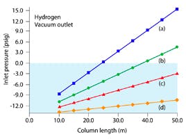
I also need to know the pressure within the inlet to estimate backflash, and for this I can also use a calculator to estimate both the inlet head pressure and column linear velocity and flow from the given method parameters. Figure 1 shows the results of these computations.

Figure 1: Calculation of required inlet pressure under the method conditions shown (Top) and the resulting vapour volume from a 1µl injection of ethyl acetate.
Figure 1 shows several important areas for consideration when evaluating GC-MS methods, starting with the inlet pressure required to generated the specified column flow rate.
When using MS detectors, it’s important to check the required inlet pressure with ‘vacuum’ selected as the outlet pressure. In this case, the combination of the desired carrier gas flow rate and column dimensions with vacuum at the column outlet gives a head pressure of 9.785 psi and a carrier gas linear velocity of 39.9 cm/sec, both of which are reasonable. Here I’m considering any values above 5psi for the inlet pressure and between 20 and 50 cm/sec for the carrier gas linear velocity to be reasonable. When using lower flow rates and larger internal diameter GC columns (typically 0.32mm i.d. or greater), the inlet pressure required to generate the selected flow rate is very low, as the vacuum is creating a flow within the column without applying any forward pressure to the carrier gas, and the electronic pneumatic control units may struggle to attain or maintain the very inlet low pressures required to generate the required column flow rate or linear velocity.
Figure 1 also shows us that under the experimental conditions, the volume of vapour which will be created in the liner by a 1 µL sample injection is around 278 mL or 32% of its total usable volume. To be absolutely sure of avoiding backflash, I like to keep the vapour volume below half of the liner capacity, although we could easily increase the injection volume to 2 µL without risking backflash, depending upon the required sensitivity of the method. Of course, this parameter will need to be empirically optimized as it was not stated within the method.
It is worth noting here the GC column chemistry cited in the method, (35%-phenyl)-methylpolysiloxane (inert and MS compatible). There are many ‘MS compatible’ phases available these days, and essentially these are phases which show lower a lower degree of bleed. These can either be selected during manufacturers QC process as those which show the lowest bleed level within a batch of columns, or the phase chemistry itself may have been altered, or the phase deactivation process improved, in order to inherently produce a lower bleed column, and hence reduce the amount of ion source fouling which occurs as a result of this bleed. Needless to say, where the phase chemistry has been altered, there may be subtle differences in selectivity between the MS compatible and non-MS compatible versions of the same nominal phase chemistry, Wherever possible, one should try to match the column chemistry to that cited in the method and very often GC-MS methods will be written so that one may recognise the manufacturer of the column from the code letters used to describe the phase (in this case DB-35MS, Rtx35-MS, ZB-35, SPB-35 and so forth). Check out our handy Phase Equivalency Table Here. MS compatibility of the GC column will generally lead to longer intervals between MS detector ion source cleaning.
As the analyte passes through the instrument it will elute into the ion source of the mass spectrometer. We have been supplied temperature values for the ion source and quadrupole, which is helpful and these values are very often omitted from method specification. Remember that we wish to keep any analytes entering the mass spectrometer in the gas phase, and that most detectors will have optimal temperatures for the various regions within the instrument, and therefore these temperatures are vital information. We have not however been provided a temperature value for the heated transfer line which carries the analytes from the end of the GC column into the detector ion source. Typically there should be a temperature differential which will step down from the transfer line, through the ion source and into the quadrupole. It is vital that less volatile analytes do not condense within the transfer line and therefore this value is typically set a little higher than the ion source temperature and a little lower than the upper temperature of the oven temperature program. In this case a value of 270 or 280 °C would be suitable.
We have also been provided an acquisition mode for the detector (in this case full scanning rather than selection ion monitoring mode) and range of masses over which the scan will be performed during each cycle of the analyser (65 to 600 m/z). Whilst the details of the analyser operation is a little beyond the scope of our present discussion (See reference [1] for further information on the working principle of the quadrupole mass analyser), we need to carefully consider for each method, the operating mode and range of the mass analyser. In full scanning mode, the detector progressively cycles from high to low mass values, and will record all ions which pass through the analyser at sequentially lower m/z values. Having a wide scan range will decrease the number of cycles per second that the detector can achieve and therefore will reduce the analyser sensitivity. Further, as our analytes will not generate ions at every m/z value, some of the acquisition will be ‘dead time’ where no signal is produced for the analytes of interest. For this reason, the scan range should be kept as narrow as possible and to within the range of molecular weights covered by the analytes of interest, if this is known. The positive benefit of full scanning is that no information is lost and all analytes within this stipulated mass range will be recorded, which is advantageous when one does not know the nature of the sample.
The alternative acquisition mode is to select target ions which are known to be present in the spectra of the analytes of interest and to ‘fix’ the analyser at these values according to the time at which the analytes elute from the column. In this way, detector cycle times are reduced and only ions know to be present are recorded, hence improving the sensitivity of the detector. When selected ion monitoring modes are used, it is important that the specification includes the m/z values of the ions being monitored, the time window over which these ions are monitored prior to switching to a new group of ions and, crucially, the dwell time for each ion, which corresponds to the amount of time within each measurement cycle that the instrument is ‘tuned’ to each of the ions within each group. A typical example of this might be;
| Ion Group | Ions (m/z) | Ion Group Time Window (mins) | Dwell Time (mS) |
| 1 | 291 | 6.1 - 6.7 | 50 |
| 1 | 182 | 6.1 - 6.7 | 75 |
| 1 | 94 | 6.1 - 6.7 | 50 |
| 2 | 134 | 6.7 - 7.1 | 60 |
| 2 | 91 | 6.7 - 7.1 | 90 |
| 2 | 56 | 6.7 - 7.1 | 90 |
Table 1: Typical method specification for quadrupole analyser settings in a selected ion monitoring type experiment.
In the method under consideration here, it is presumed that the range of 65 of 600 m/z has been optimized to include the analytes of interest, although this should be fully confirmed prior to transferring the method into your laboratory. If low molecular weight analytes are present within the sample or analytes are known to produce significant fragments at low molecular weight, then one might consider lowering the lower bound of the range. Similarly, if high molecular weight analytes are being analysed, then the upper limit of the range should be increased. Typically, not much useful information will be gained below around 30 m/z and some modern quadrupole analysing devices will have a maximum upper mass range of 2000 m/z.
The solvent delay value (7 mins.) corresponds to the time when the filaments used to generate fragmenting electrons within the ion source are switched off, and therefore no spectral information (and therefore no chromatogram) is being generated. The solvent delay time is used to protect the filaments during the time when the sample solvent is eluting from the analytical column, which causes a reduction in vacuum within the ion source and may ‘burn out’ the filaments within the instrument. This delay time can also be used to save filament burn time (filaments have a finite lifetime) prior to the time at which the first analytes begin to elute from the GC column. In this method then, we are assuming that no useful information is derived for the first seven minutes of the analysis, which will need to be verified. This value also suggests that some optimization of the temperature program could have been possible to save wasted time at the beginning of each analysis. One needs to take care when optimizing the solvent delay time and if the mass spectrometer is fitted with a vacuum monitoring gauge the increase in source pressure followed by the subsequent reduction can be used to gauge the passage of the sample solvent through the ion source, and can therefore be used to set an appropriate solvent delay.
This brings us to the final consideration, that of the instrument ‘tune’. In this case the name of the type of tune has been cited as ‘Autotune’. It is worthy of note that this is a particular tune file associated with a particular manufacturer and the tune itself will impart certain response characteristics to the instrument, depending on the tune targets written into the instrument tune algorithm. Some tune algorithms may be good for overall spectral fidelity, some may target higher sensitivity at higher or lower mass, some may be tunes for specific types of target analytes or application areas such as environmental analysis. When implementing a literature method or transferring methods between laboratories and instruments, one needs to carefully consider the instrument tuning and assess it’s appropriateness for the analysis at hand. Whilst a full consideration of the various aspects of MS detector tuning is beyond our scope here, it is important that the analyst understands the tune parameters in order to make a judgement regarding the suitability of the instrument tuning. Some tunes are more suited to qualitative analysis and others for quantitative analysis for example.
Whilst all manufacturers will differ in the tune targets they apply to instrument variables for the various methods of tuning, they will all result in an assurance that the instrument is operating to within required tolerances. For this reason, I tend to prefer a more objective measurement to be included in method specifications, and some typical values that might be included are;
MS resolution – m/z 69 (perflurotributylamine) has a peak width of between 0.5 and 0.6 m/z
MS Sensitivity – m/z 502 (perflurotributylamine) has a signal count of least X with a signal to noise value of Y OR analyte X injected at 0.1 µg/ML has a signal to noise ratio of at least 5:1
For more information on setting and interpreting MS tuning parameters see Reference [2]
When evaluating GC-MS methods, it’s important to consider the suitability of the column dimensions and required carrier gas flow rate to establish the feasibility of easily meeting and maintaining the lower inlet pressures required when the GC column outlet is at vacuum.
The correct setting of more minor variables within the MS detector is also important to ensure that the detector performance requirements are met. Giving prior consideration to the method variables and thinking through any potential issues can save a lot of head scratching once we have crossed the laboratory threshold!
Related articles