10 Jan 2019
HPLC method development critical decisions
Do you ever look with envy at other labs and think ‘I wish we were equipped with such a sophisticated and effective HPLC method development system’?
Systems that are equipped with several columns, eluent reservoirs, and columns switching valves that are connected to automated software — these labs are the labs that can test a wide number of column and eluent combinations, in order to find the best conditions during the initial phase of method development.
While these advanced systems are flashy and efficient, they don’t present a universal panacea in HPLC method development — a simple, pared-down approach can still achieve a great deal. In my experience, a well-designed single screening experiment can reveal a lot about the sample at hand and inform future method choices. However, I also find that interpretations of initial screen results are regularly where less experienced method developers get stuck.
Never fear — this article aims to help. In it, you’ll find some simple scenarios to guide you through the next steps. Over the years, I’ve designed some robust decision trees that can aid future experimentation as, together, we progress through the method development paradigm. These trees are designed to maximise return on effort — so that simple experiments can be tried and tested before more complex experiments or time-consuming steps are undertaken.
Step 1 – Arrange your screening experiment to shoot for k* (let’s call that an Average Gradient Retention Factor) of around 5.
The formula we use here is;
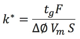
tg is the gradient time in minutes, F is the eluent flow rate in mL/min, ΔΦ is the change in eluent composition (i.e. 0.4 for a 20 to 60% B gradient), Vm is the interstitial volume of the column, which is estimated by;
S is a shape selectivity factor which can be estimated by, 0.25 Mw0.5 (for analytes < 1000Da a value of 5 is typically used for S)
Some of this is predicated on the column dimensions used which determines Vm, and some of the more common column dimensions give the following interstitial column volumes (all calculated using Equation 2);
| Column Dimensions (mm) | Interstitial Volume (Vm) (mL) |
|
150 x 4.6 100 x 4.6 100 x 2.1 50 x 2.1 |
1.7 1.1 0.24 0.12 |
Table 1: Interstitial Column Volumes (Vm) for various popular HPLC column dimensions.
For screening experiments – we like a nice wide gradient range to take care of the various polarities of analyte that we might encounter, so let’s say a range of 0.8 which will mean setting the gradient from 10%B to 90%B (not forgetting that the we hold the gradient at 90% for a considerable time to assess if there are any really strongly retained analytes).
I’m going to assume an eluent flow rate of 1.0 mL/min for the 4.6mm internal diameter columns and 0.5 mL/min for the 2.1 mm internal diameter columns.
Armed with all this information we can re-arrange Equation 1 to give us a gradient time figure which will result in a k* value of 5 for each of the columns shown in Table 1;
Calculating for each of the column volume and flow rate combinations gives gradient times shown in Table 2.
|
Column Dimensions (mm) |
Interstitial Volume (Vm) (mL) |
Flow rate (mL) |
Gradient Time (for k*=5) (mins) |
|
150 x 4.6 100 x 4.6 100 x 2.1 50 x 2.1 |
1.7 1.1 0.24 0.12 |
1.0 1.0 0.5 0.5 |
34 22 9.6 4.8 |
Each value calculated using a shape factor (S) of 5.
Table 2: Gradient times required to achieve a k* of 5 for various combinations of HPLC column volume, eluent flow rate and gradient range.
So now we have gathered some useful information and we can consider undertaking our initial experiments – I’ve proposed below a set of conditions based on a good quality C18 column, however if you know something of the physical chemical properties of your analyte, you may want to choose a more appropriate column chemistry (see Ref 1 and 2 for more details) or eluent pH value;
| Column: | C18 (150 x 4.6mm) | ||||||||
| Eluent: | [A] MeCN [B] Water [C] 2% TFA v/v 200mM Ammonium Acetate (aq) using the following gradient table | ||||||||
| Gradient: | 10% to 80% in 34 minutes (see Table 2 for Gradient Time details)
(use an initial hold time (5% of the gradient time) if the method is expected to be transferred to different equipment or laboratories for dwell volume matching)
Here we have opted for an acidic mobile phase at constant ionic strength (0.1% v/v TFA, 10mM ammonium acetate) which will very much help in the interpretation of where to go next when we obtain the results from the initial screening experiment. |
||||||||
| Flow Rate: | 1 mL/min (for this column volume – see Table 2 for relevant details for other column dimensions) |
||||||||
| Diluent: | 10% MeCN (aq) (or as close as possible to this concentration given solubility constraints, to avoid peak shape deformation) |
||||||||
| Detection: | Electrospray API -MS in pos/neg switching mode if possible or UV detection at an appropriate wavelength for the sample type (choose 254 nm if the analyte chemistry is unknown) |
Ok – so let’s assume we have undertaken our initial screening experiments, so what do we do with the results, as unless you are extremely lucky, you are unlikely to get a perfect separation from the screening experiment – and if you do, you can write to me and let me know!
I’m going to outline a few typical scenarios here and then show you some very simple logic flows and decision trees to follow in order to make the most efficient use of your method development time. The principle here is that we are adopting a ‘kill quickly’ policy and performing a limited number of experiments post the initial screen before stopping optimisation and changing to a new column. This avoids the funnel of diminishing returns, where one is tempted to perform an (often long) series of ‘tweaks’ in order to achieve a satisfactory separation. This latter approach is both time consuming a rarely leads to robust HPLC methods and the kill quickly philosophy is much more time efficient in the long run.
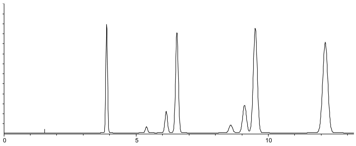
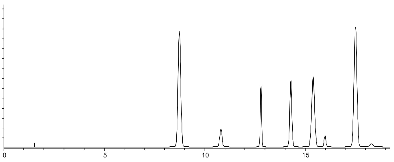
In this simulated experiment we are separating a mixture of 5 pharmaceutical test compounds and three impurity peaks. We can expect the test compounds to be at a higher concentration than any of the impurities.
Scenario 1: Some of my peaks are missing
Only 7 of the 8 expected peaks can be seen in the chromatogram
Reasons:
- Irreversible or very long retention (see Scenario 3)
- Co-elution (see scenario 5)
- No or poor analyte retention (see Scenario 2)
Actions:
- Investigate elongated retention by repeating the screening with a hold at the end of the chromatogram the same length as the gradient time used – examine the isocratic hold section for the missing peak
- Proceed to Reasons 2 & 3
Scenario 2: All peaks elute very quickly
Reasons:
- Poor interaction between analyte and stationary phase (possibly due to polarity mismatch between analyte and stationary phase)
Actions:
- Run two further experiments at pH 5.0 and 7.5 and assess retention behaviour
- Increased retention indicates one or more strongly basic analytes – consider further optimising pH if k values (calculated using Equation 4) are between 1 and 15 (ideally between 2 and 10).
Where tr is the analyte retention time and t0 is the system hold-up time (dead volume)
Note that the use of retention factor (k) values within gradient analysis is not strictly indicative of retention behaviour but these figures can be used as a rough guide to the applicability of the method - If any analytes remain at k = 2 or below, consider switching to a different Stationary Phase
Scenario 3: All peals elute very slowly
Reasons:
- Interaction between analytes and stationary phase is too strong, due to the analytes being extremely hydrophobic (high LogP values)
Actions:
- If all peaks elute within the isocratic portion at the end of the gradient, consider changing to a less retentive column (C8 / C4, Phenyl etc.) or altering the eluent pH
- Repeat the experiment at pH 5.5 and 7.5 and assess the retention behaviour – go to step 3
- If most of the analytes elute within the gradient time, either after the initial screen or the pH adjustment experiments, calculate the elution composition at which the first peak elutes (remember to account for any system gradient dwell volume) and subtract 20%B.
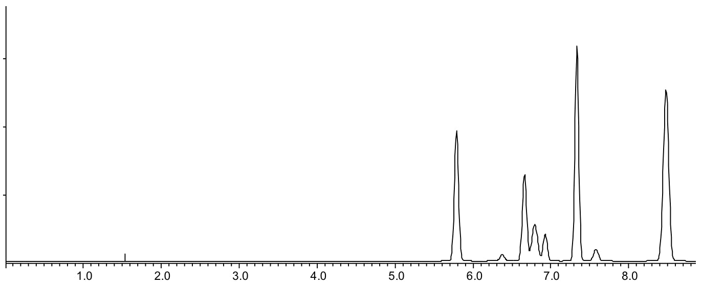
- Carry out a further experiment starting at the gradient composition calculated in step 3 but with the same gradient rate as the starting experiment (%B change / minute) – in this case the first peak elutes at approximately 75% B therefore the gradient will start at 50% and the rate of change from the original screen is 2.5%B per minute. Therefore, the new gradient will be 50%B to 90% in 16 minutes.
- It this produces more reasonable retention times, consider optimising gradient slope by having and doubling the gradient rate (1.25%B per minute, 50%B to 90%B in 32 minutes and 5% per minute, 50%B to 90%B in 8 minutes) and estimate the best gradient slope (rate) using the three chromatograms obtained at 1.25, 2.5 and 5%B/min.
Same sample separated using 50 – 85% B in 20 mins pH 5.5
Scenario 4: Peaks show wide range of retention behaviours
Reasons:
- Analytes have a wide range of LogP or LogD values and therefore show widely different interaction with the stationary phase. This can be due to the native hydrophobicity of the analytes or that hydrophobicity is modified by the presence of ionisable groups and the extent of ionisation, which is controlled by eluent pH
Actions:
- Double the gradient rate to 5%B per minute (i.e. 10%B to 90%B in 16 minutes) and estimate the best gradient slope between 2.5%B and 5.0%B per minute. Exercise extreme caution when evaluating co-elution and ensure that peaks are tracked either by peak area or UV spectral identification or using MS detection.
- Ideal retention factor range (see Equation 4) is between 2 and 10
- If no suitable gradient slope can be estimated, repeat the initial screening experiment at pH 5.0 and 7.5 to assess the possibility for pH optimisation
- If no combination of gradient slope and pH can be identified for a suitable separation, consider changing to a different stationary phase and repeat the initial screening exercise.
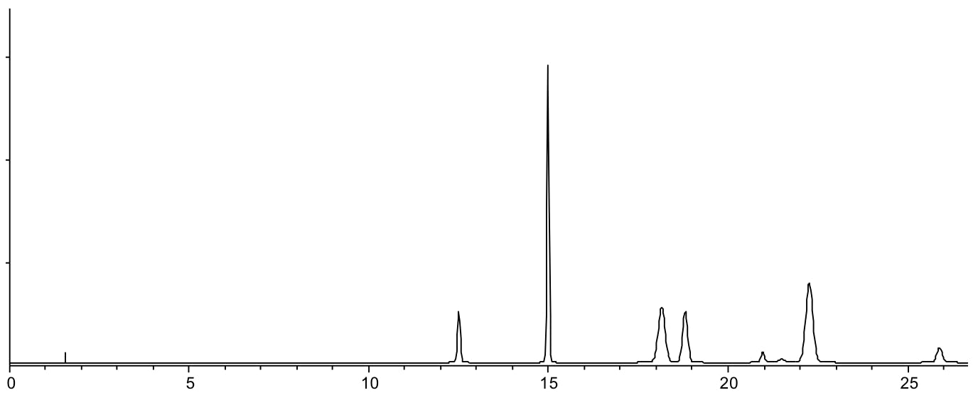
Chromatogram resulting from gradient slope of 5% per minute at pH 5.5. Whilst further development is required to improve resolution (and robustness), all peaks are separated within a reasonable retention range.
Scenario 5: Co-elution in the middle of the chromatogram / compressed retention range
Reasons:
- Analytes have similar LogP or LogD values and are interacting with the stationary phase in a similar fashion
Actions:
- Calculate the eluent composition at the elution time of the first peak at subtract 10%B (in this case the first peak elutes at around 20% B therefore the gradient would start at 5% B)
- Halve the gradient rate from the original screening separation (from 2.5%B per minute to 1.25%B per minute) so the gradient would new be 5%B to 90%B in 60 minutes (approximately)
- Assess the new chromatogram and estimate a suitable gradient slope (%B/min) and upper %B limit for the method. Exercise extreme caution when evaluating co-elution and ensure that peaks are tracked either by peak area or UV spectral identification or using MS detection.
- If a suitable gradient range cannot be identified – consider changing to Methanol as an alternative modifier using the initial screening conditions for the first experiment and re-start at Number 1 in this list.
- Whilst it may be tempting to use pH to optimise the separation prior to the above steps, when peaks are compressed as shown here, it will be very difficult to find an optimum pH and the method is likely to be non-robust. Once a suitable gradient slope and modifier have been achieved, the peaks should elute over a wider retention range and pH optimisation should be possible. Further experiments at pH 5.5 and 7.5 will enable an estimation of the optimal pH from the 3 chromatograms obtained (pH 2.1, 5.5 and 7.5).
- If a suitable separation cannot be achieved, select a more suitable HPLC column and repeat the initial screening exercise.
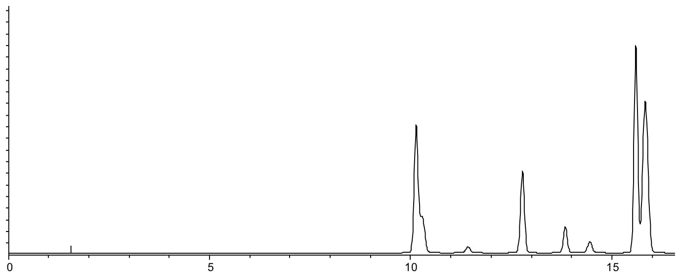
Same separation carried using a shallow gradient 30 – 65 %B in 30 minutes.
Scenario 6: Co-elution at the start and end (or throughout) the chromatogram
Reasons:
- Analytes have similar LogP or LogD values and are interacting with the stationary phase in a similar fashion
- Co-elution over the whole chromatogram indicates many similar species or sub-optimal selectivity, indicating a change is required to the stationary phase or eluent
Actions:
- Calculate the eluent composition at the elution time of the first peak at subtract 10%B (in this case the first peak elutes at around 20% B therefore the gradient would start at 5% B)
- Switch to Methanol as the modifier and repeat the screening exercise but starting the gradient at the composition calculated in step 1 – assess if the degree or number of co-elutions has improved. Move to step 3 with either acetonitrile or methanol.
- Repeat the screening separation at pH5.5 – does the selectivity change significantly? If so – conduct a further experiment at pH 7.5, if not consider a change to a different stationary phase
- From the three pH experiments, pH 2.1, 5.5 and 7.5 you will be able to estimate a suitable pH for the separation. If no suitable pH can be identified, consider using a stationary phase capable of withstanding high eluent pH and repeat the experiment at pH10. Re-evaluate the chromatography to assess if a pH between 7.5 and 10 might be suitable for the separation. If suitable separation cannot be achieved, consider using a stationary phase with an alternative selectivity (see references 1 and 2).
Same separation carried out using Methanol as the modifier at pH 6.5.
Whilst in almost all cases, further optimisation work will be required at the end of each process, the order in which changes are undertaken and the types of change will lead to a significant reduction in effort for those developing separations without the aid of optimisation software!
References;
- Do you really know your stationary phase chemistry?
-
Relating Analyte Properties to HPLC Column Selectivity the road to Nirvana
Do you ever look with envy at other labs and think ‘I wish we were equipped with such a sophisticated and effective HPLC method development system’?
Systems that are equipped with several columns, eluent reservoirs, and columns switching valves that are connected to automated software — these labs are the labs that can test a wide number of column and eluent combinations, in order to find the best conditions during the initial phase of method development.
While these advanced systems are flashy and efficient, they don’t present a universal panacea in HPLC method development — a simple, pared-down approach can still achieve a great deal. In my experience, a well-designed single screening experiment can reveal a lot about the sample at hand and inform future method choices. However, I also find that interpretations of initial screen results are regularly where less experienced method developers get stuck.
Never fear — this article aims to help. In it, you’ll find some simple scenarios to guide you through the next steps. Over the years, I’ve designed some robust decision trees that can aid future experimentation as, together, we progress through the method development paradigm. These trees are designed to maximise return on effort — so that simple experiments can be tried and tested before more complex experiments or time-consuming steps are undertaken.
Step 1 – Arrange your screening experiment to shoot for k* (let’s call that an Average Gradient Retention Factor) of around 5.
The formula we use here is;
tg is the gradient time in minutes, F is the eluent flow rate in mL/min, ΔΦ is the change in eluent composition (i.e. 0.4 for a 20 to 60% B gradient), Vm is the interstitial volume of the column, which is estimated by;
S is a shape selectivity factor which can be estimated by, 0.25 Mw0.5 (for analytes < 1000Da a value of 5 is typically used for S)
Some of this is predicated on the column dimensions used which determines Vm, and some of the more common column dimensions give the following interstitial column volumes (all calculated using Equation 2);
| Column Dimensions (mm) | Interstitial Volume (Vm) (mL) |
|
150 x 4.6 100 x 4.6 100 x 2.1 50 x 2.1 |
1.7 1.1 0.24 0.12 |
Table 1: Interstitial Column Volumes (Vm) for various popular HPLC column dimensions.
For screening experiments – we like a nice wide gradient range to take care of the various polarities of analyte that we might encounter, so let’s say a range of 0.8 which will mean setting the gradient from 10%B to 90%B (not forgetting that the we hold the gradient at 90% for a considerable time to assess if there are any really strongly retained analytes).
I’m going to assume an eluent flow rate of 1.0 mL/min for the 4.6mm internal diameter columns and 0.5 mL/min for the 2.1 mm internal diameter columns.
Armed with all this information we can re-arrange Equation 1 to give us a gradient time figure which will result in a k* value of 5 for each of the columns shown in Table 1;
Calculating for each of the column volume and flow rate combinations gives gradient times shown in Table 2.
|
Column Dimensions (mm) |
Interstitial Volume (Vm) (mL) |
Flow rate (mL) |
Gradient Time (for k*=5) (mins) |
|
150 x 4.6 100 x 4.6 100 x 2.1 50 x 2.1 |
1.7 1.1 0.24 0.12 |
1.0 1.0 0.5 0.5 |
34 22 9.6 4.8 |
Each value calculated using a shape factor (S) of 5.
Table 2: Gradient times required to achieve a k* of 5 for various combinations of HPLC column volume, eluent flow rate and gradient range.
So now we have gathered some useful information and we can consider undertaking our initial experiments – I’ve proposed below a set of conditions based on a good quality C18 column, however if you know something of the physical chemical properties of your analyte, you may want to choose a more appropriate column chemistry (see Ref 1 and 2 for more details) or eluent pH value;
| Column: | C18 (150 x 4.6mm) | ||||||||
| Eluent: | [A] MeCN [B] Water [C] 2% TFA v/v 200mM Ammonium Acetate (aq) using the following gradient table | ||||||||
| Gradient: | 10% to 80% in 34 minutes (see Table 2 for Gradient Time details)
(use an initial hold time (5% of the gradient time) if the method is expected to be transferred to different equipment or laboratories for dwell volume matching)
Here we have opted for an acidic mobile phase at constant ionic strength (0.1% v/v TFA, 10mM ammonium acetate) which will very much help in the interpretation of where to go next when we obtain the results from the initial screening experiment. |
||||||||
| Flow Rate: | 1 mL/min (for this column volume – see Table 2 for relevant details for other column dimensions) |
||||||||
| Diluent: | 10% MeCN (aq) (or as close as possible to this concentration given solubility constraints, to avoid peak shape deformation) |
||||||||
| Detection: | Electrospray API -MS in pos/neg switching mode if possible or UV detection at an appropriate wavelength for the sample type (choose 254 nm if the analyte chemistry is unknown) |
Ok – so let’s assume we have undertaken our initial screening experiments, so what do we do with the results, as unless you are extremely lucky, you are unlikely to get a perfect separation from the screening experiment – and if you do, you can write to me and let me know!
I’m going to outline a few typical scenarios here and then show you some very simple logic flows and decision trees to follow in order to make the most efficient use of your method development time. The principle here is that we are adopting a ‘kill quickly’ policy and performing a limited number of experiments post the initial screen before stopping optimisation and changing to a new column. This avoids the funnel of diminishing returns, where one is tempted to perform an (often long) series of ‘tweaks’ in order to achieve a satisfactory separation. This latter approach is both time consuming a rarely leads to robust HPLC methods and the kill quickly philosophy is much more time efficient in the long run.
In this simulated experiment we are separating a mixture of 5 pharmaceutical test compounds and three impurity peaks. We can expect the test compounds to be at a higher concentration than any of the impurities.
Scenario 1: Some of my peaks are missing
Only 7 of the 8 expected peaks can be seen in the chromatogram
Reasons:
- Irreversible or very long retention (see Scenario 3)
- Co-elution (see scenario 5)
- No or poor analyte retention (see Scenario 2)
Actions:
- Investigate elongated retention by repeating the screening with a hold at the end of the chromatogram the same length as the gradient time used – examine the isocratic hold section for the missing peak
- Proceed to Reasons 2 & 3
Scenario 2: All peaks elute very quickly
Reasons:
- Poor interaction between analyte and stationary phase (possibly due to polarity mismatch between analyte and stationary phase)
Actions:
- Run two further experiments at pH 5.0 and 7.5 and assess retention behaviour
- Increased retention indicates one or more strongly basic analytes – consider further optimising pH if k values (calculated using Equation 4) are between 1 and 15 (ideally between 2 and 10).
Where tr is the analyte retention time and t0 is the system hold-up time (dead volume)
Note that the use of retention factor (k) values within gradient analysis is not strictly indicative of retention behaviour but these figures can be used as a rough guide to the applicability of the method - If any analytes remain at k = 2 or below, consider switching to a different Stationary Phase
Scenario 3: All peals elute very slowly
Reasons:
- Interaction between analytes and stationary phase is too strong, due to the analytes being extremely hydrophobic (high LogP values)
Actions:
- If all peaks elute within the isocratic portion at the end of the gradient, consider changing to a less retentive column (C8 / C4, Phenyl etc.) or altering the eluent pH
- Repeat the experiment at pH 5.5 and 7.5 and assess the retention behaviour – go to step 3
- If most of the analytes elute within the gradient time, either after the initial screen or the pH adjustment experiments, calculate the elution composition at which the first peak elutes (remember to account for any system gradient dwell volume) and subtract 20%B.
- Carry out a further experiment starting at the gradient composition calculated in step 3 but with the same gradient rate as the starting experiment (%B change / minute) – in this case the first peak elutes at approximately 75% B therefore the gradient will start at 50% and the rate of change from the original screen is 2.5%B per minute. Therefore, the new gradient will be 50%B to 90% in 16 minutes.
- It this produces more reasonable retention times, consider optimising gradient slope by having and doubling the gradient rate (1.25%B per minute, 50%B to 90%B in 32 minutes and 5% per minute, 50%B to 90%B in 8 minutes) and estimate the best gradient slope (rate) using the three chromatograms obtained at 1.25, 2.5 and 5%B/min.
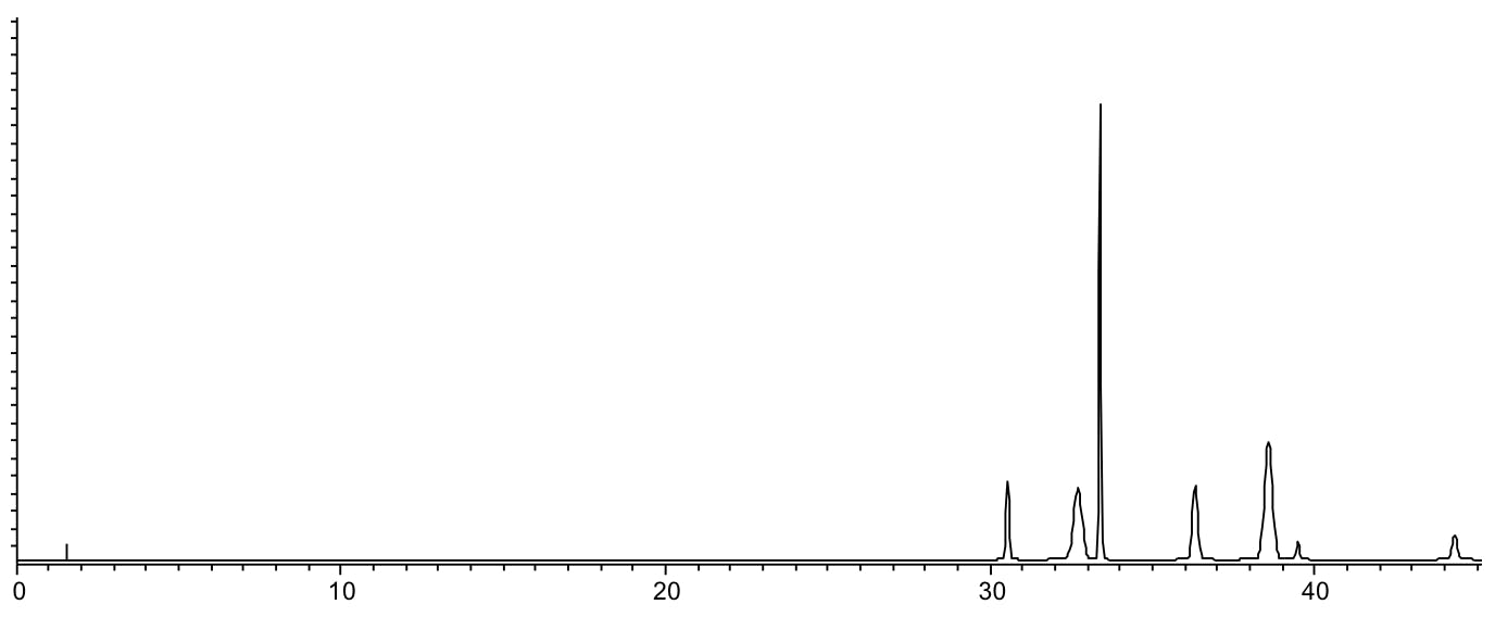
Same sample separated using 50 – 85% B in 20 mins pH 5.5
Scenario 4: Peaks show wide range of retention behaviours
Reasons:
- Analytes have a wide range of LogP or LogD values and therefore show widely different interaction with the stationary phase. This can be due to the native hydrophobicity of the analytes or that hydrophobicity is modified by the presence of ionisable groups and the extent of ionisation, which is controlled by eluent pH
Actions:
- Double the gradient rate to 5%B per minute (i.e. 10%B to 90%B in 16 minutes) and estimate the best gradient slope between 2.5%B and 5.0%B per minute. Exercise extreme caution when evaluating co-elution and ensure that peaks are tracked either by peak area or UV spectral identification or using MS detection.
- Ideal retention factor range (see Equation 4) is between 2 and 10
- If no suitable gradient slope can be estimated, repeat the initial screening experiment at pH 5.0 and 7.5 to assess the possibility for pH optimisation
- If no combination of gradient slope and pH can be identified for a suitable separation, consider changing to a different stationary phase and repeat the initial screening exercise.
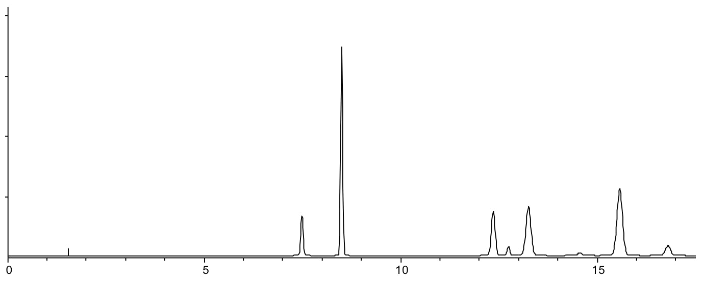
Chromatogram resulting from gradient slope of 5% per minute at pH 5.5. Whilst further development is required to improve resolution (and robustness), all peaks are separated within a reasonable retention range.
Scenario 5: Co-elution in the middle of the chromatogram / compressed retention range
Reasons:
- Analytes have similar LogP or LogD values and are interacting with the stationary phase in a similar fashion
Actions:
- Calculate the eluent composition at the elution time of the first peak at subtract 10%B (in this case the first peak elutes at around 20% B therefore the gradient would start at 5% B)
- Halve the gradient rate from the original screening separation (from 2.5%B per minute to 1.25%B per minute) so the gradient would new be 5%B to 90%B in 60 minutes (approximately)
- Assess the new chromatogram and estimate a suitable gradient slope (%B/min) and upper %B limit for the method. Exercise extreme caution when evaluating co-elution and ensure that peaks are tracked either by peak area or UV spectral identification or using MS detection.
- If a suitable gradient range cannot be identified – consider changing to Methanol as an alternative modifier using the initial screening conditions for the first experiment and re-start at Number 1 in this list.
- Whilst it may be tempting to use pH to optimise the separation prior to the above steps, when peaks are compressed as shown here, it will be very difficult to find an optimum pH and the method is likely to be non-robust. Once a suitable gradient slope and modifier have been achieved, the peaks should elute over a wider retention range and pH optimisation should be possible. Further experiments at pH 5.5 and 7.5 will enable an estimation of the optimal pH from the 3 chromatograms obtained (pH 2.1, 5.5 and 7.5).
- If a suitable separation cannot be achieved, select a more suitable HPLC column and repeat the initial screening exercise.
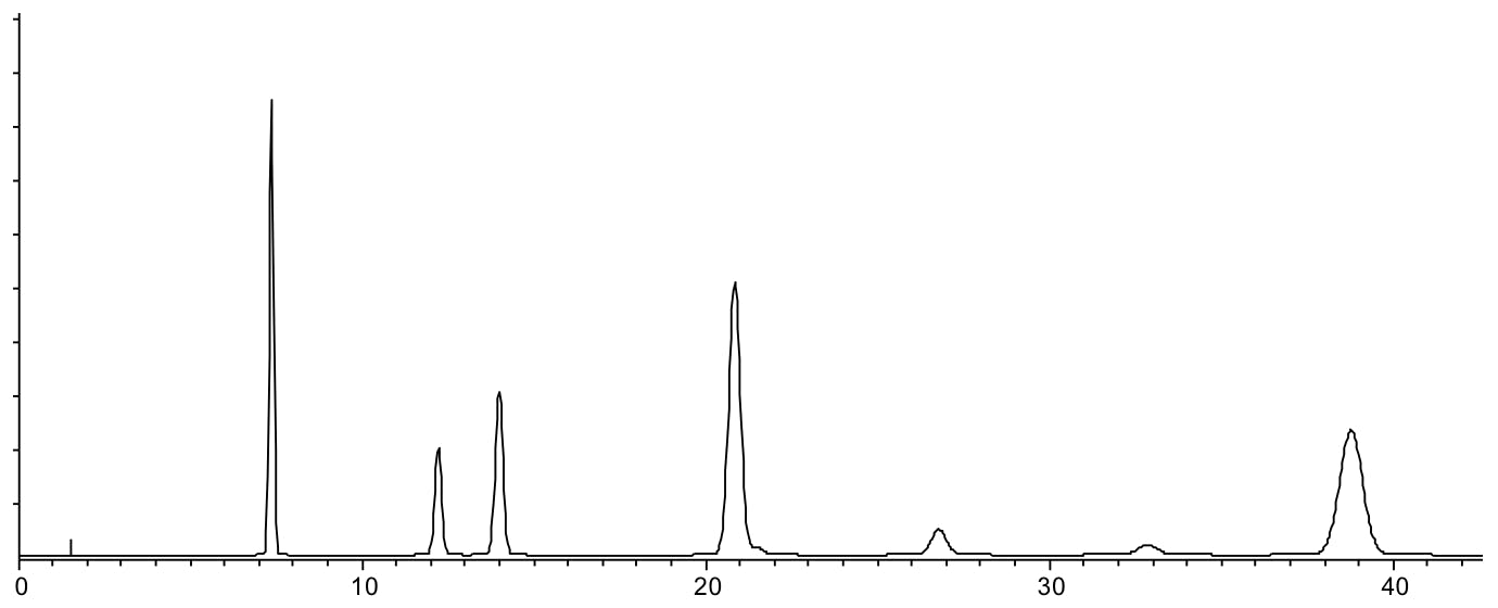
Same separation carried using a shallow gradient 30 – 65 %B in 30 minutes.
Scenario 6: Co-elution at the start and end (or throughout) the chromatogram
Reasons:
- Analytes have similar LogP or LogD values and are interacting with the stationary phase in a similar fashion
- Co-elution over the whole chromatogram indicates many similar species or sub-optimal selectivity, indicating a change is required to the stationary phase or eluent
Actions:
- Calculate the eluent composition at the elution time of the first peak at subtract 10%B (in this case the first peak elutes at around 20% B therefore the gradient would start at 5% B)
- Switch to Methanol as the modifier and repeat the screening exercise but starting the gradient at the composition calculated in step 1 – assess if the degree or number of co-elutions has improved. Move to step 3 with either acetonitrile or methanol.
- Repeat the screening separation at pH5.5 – does the selectivity change significantly? If so – conduct a further experiment at pH 7.5, if not consider a change to a different stationary phase
- From the three pH experiments, pH 2.1, 5.5 and 7.5 you will be able to estimate a suitable pH for the separation. If no suitable pH can be identified, consider using a stationary phase capable of withstanding high eluent pH and repeat the experiment at pH10. Re-evaluate the chromatography to assess if a pH between 7.5 and 10 might be suitable for the separation. If suitable separation cannot be achieved, consider using a stationary phase with an alternative selectivity (see references 1 and 2).
Same separation carried out using Methanol as the modifier at pH 6.5.
Whilst in almost all cases, further optimisation work will be required at the end of each process, the order in which changes are undertaken and the types of change will lead to a significant reduction in effort for those developing separations without the aid of optimisation software!
References;
- Do you really know your stationary phase chemistry?
-
Relating Analyte Properties to HPLC Column Selectivity the road to Nirvana
Related articles