19 May 2021
Killer Gas Chromatography variables and other insidious ways to destroy your chromatography!
By Tony Taylor
Most readers will be familiar with the major GC variables, setting them into our data acquisition software and reading them from our SOP’s or Laboratory Work instruction methods on a regular basis. Generally speaking, those variables are not in scope here, other than to consider the lesser understood effects of some of them.
Instead, I’d like to concentrate on variables which can really impact our chromatography, but may be on hidden, supplementary or advanced pages of our software, or which may appear on the main software acquisitions menus but are poorly understood or rarely altered. These variables are often not specifically referenced in laboratory methods documents or, if they do appear, are poorly understood. Whilst some of these variables appear to be esoteric, I’ve seen all of these either ruin otherwise perfectly good chromatography or confound users during method troubleshooting.

Autosampler Syringe Plunger Speed & Needle Depth – most autosamplers will give the option to change the speed of the plunger within the syringe barrel, both during sample aspiration and injection into the GC. When dealing with viscous samples, the plunger speed is usually set to a slower speed in order to avoid cavitation of the sample within the needle and hence variable sample amounts being aspirated. The syringe needle depth may also need to be adjusted when dealing with very low sample amounts, vials with different shapes or multiphasic samples, for example, where the top layer of a biphasic solvent mixture needs to be sampled. The speed of sample ejection into the inlet may also need to be altered with narrow bore inlet liners or some modes of cool on column injection.
Wash solvents – certainly not the most exciting of topics within the GC arena, but highly important none the less. Wash solvents should be chosen on their ability to solubilise the analytes of interest and not just the sample matrix, this fact is often overlooked when choosing appropriate solvents. The solvents should be highly miscible with the GC injection solvent and, where possible, two wash solvent bottles should be used, one ‘dirtier’ and one ‘cleaner’ bottle. The trick is to wash the syringe prior to sample aspiration in the cleaner solvent and post injection to wash first in the dirtier solvent followed by a rinse in the cleaner solvent. Where three wash solvent positions are available, then the third solvent should be reserved for the pre-sample aspiration wash only. It’s also a good idea to leave wash solvent bottles uncapped as any sample residue from the outside of the syringe needle can potentially contaminate the septum or needle guide from the bottle tops, and be resolubilised into the next sample, causing carryover. Always try to aspirate the wash solvent and discard to waste three times in each operation and ensure that the syringe needle does not penetrate any liquid in the waste bottle - i.e. empty the wate bottle regularly! Having a table of conditions within the method which stipulates the wash regime is a great way to highlight the importance of this variable;
| Wash A | Wash B | Sample | |
| Pre-Injection | 10μL discard to waste (x3) | ||
| Injection | 10μL discard to waste (x3) | ||
| Pump 5μL x 3 | |||
| Aspirate and inject 1μL | |||
| Post-Injection | 10μL discard to waste (x3) | ||
| 10μL discard to waste (x3) |
Paying attention to the wash solvent regime will help to improve your quantitative reproducibility by cutting down on carryover from injection to injection.
Injection solvent (Sample Solvent) – again not the most inspiring of topics, however one which can be very important in determining peak shape, especially in splitless injection. I realise that most written methods will cite the injection solvent to be used, and this parameter may be reliant upon sample extraction or manipulation operations from a previous step in the analytical workflow. I cite the importance of the injection solvent here as less experienced GC users may not be aware of just how important the selection of injection solvent is. Injection solvent expansion volume plays an important role in carry over with both split and splitess injection. If the injected liquid volume results in a gas volume which exceeds the liner volume under the operating conditions employed, this will potentially contaminate the inlet and associated tubing which may result in carry over into subsequent injections. Interested readers can look up the phenomenon of ‘backflash’ for more information. In splitless injection mode, the solvent plays a major role in focussing analytes at the head of the analytical column and so peak shape in the splitless mode, especially for less volatile analytes, will rely on the compatibility of the injection solvent polarity with that of the GC column stationary phase material. Incompatibility will lead to shouldering and splitting analytes peaks.
Septum Purge Flow – the septum purge gas flows directly beneath the under face of the inlet septum and serves to carry away any outgassing products and contaminants from the septum material as well as having a role in controlling the degree of mass discrimination (relative discrimination between high and low boiling analytes) depending upon the configuration of the liner. Whilst most modern GC systems will control the septum purge flow, it is encouraged to know what this setting is and to manually check the flow prior to analysis. It wouldn’t be the first time that I’ve seen an electronic flow (or pressure) controller to be reading the incorrect value and this problem can be very difficult to troubleshoot unless one knows to look for it! Stating the required value (typically just a few mL per minute) improves awareness for less experienced staff.
Splitless Time (Purge Time) – the time at which the split vent is opened after sample injection in splitless injection mode. I only sporadically see the time associated with this variable written into analytical methods which is surprising as it can critically affect both baseline quality, peak shape of the solvent and early eluting analyte peaks as well as the quantitative reproducibility of early eluting analytes. Ideally the splitless time is empirically optimised such that the vast majority of all analytes have entered the column and only the lingering excess sample solvent is ejected via opening the split valve. The optimisation involves measuring the peak height (or area) of early eluting analytes whilst lengthening the splitless time. Too short a splitless time and the analyte peaks will continue to grow as the splitless time is lengthened, the peak area will eventually reach a constant value and the ideal splitless time (typically 0.25 to 1.25 minutes post injection) is that which is associated with the second constant peak height or area measurement. Whenever specifying a splitless time, it is necessary to also specify the split flow rate or split ratio. A high split ratio is preferred to ensure that the excess sample solvent vapours are quickly ejected from the inlet to avoid an oversize and tailing solvent peak.
Pulsed Injection Pressures and Time – in split and splitless injection it is sometimes advisable to apply a higher inlet pressure during the sample introduction phase to reduce backflash (inlet contamination due to overspilled sample vapour) or to increase injection volume for increased sensitivity. The inlet pressures and flows, as well as the time for the increased pressure phase. are very important in determining the quantitative accuracy of the method and these parameters are typically empirically optimised, based on recommended manufacturers settings. The phasing of the pressure reduction with any splitless time is also crucial. It is good practice to lay out all of these variables in a table within the method and to optimise them carefully to avoid poor analyte peak shapes and very poor quantitative reproducibility, especially for early eluting analytes.
Oven Equilibration Time – is the time between the GC oven setpoint being reached and detected by the oven thermocouple and the instrument registering a ‘ready’ state to begin the next injection in the sequence. This seemingly innocuous parameter is often ignored but can influence the selectivity and resolution of early eluting compounds and I’ve also known it to affect to the quantitative reproducibility. Essentially, just because the air within the GC oven has reached the setpoint temperature to begin the next analysis, the same is not necessarily true for the carrier gas flowing through the column, due to the thermal lag created by the capillary column walls and stationary phase. This is especially true for larger bore (internal diameter) columns and those with thicker stationary phase films. If the carrier flowing through the column has not reached thermal equilibrium with the air within the oven, the temperature gradient effectively begins at the wrong temperature, which can affect critical processes governing analyte focussing and separation, resulting in irreproducibility. Always pay attention to this parameter and extend the equilibration time if necessary, to correct any issues with peak shape (typically peak broadening of later eluting analytes) or retention time and resolution of earlier eluting analytes.
Initial Oven Temperature (Splitless Injection) – whilst all methods will cite the initial oven temperature within the temperature program, I wonder if we take the time to properly consider the importance of this parameter in splitless injection methods? To overcome gross peak broadening caused as the analyte slowly enters the column from the splitless inlet (analyte transfer typically occurs at the carrier gas flow rate), the analytes must be focussed at the head of the GC column. This is usually achieved by condensation of higher boiling analytes and solvent trapping of the lower boiling analytes. Both processes are directly affected by the initial column temperature and the general recommendation is that the initial oven temperature is 10-20 oC below the boiling point of the sample injection solvent to avoid peak broadening and shouldering. The time for which the initial oven temperature is held, can also be crucial in determining peak shape in splitless injection and is typically empirically optimised. Do all your splitless methods follow the rules? Note that the column Equilibration Time (above) can also play a role in determining the peak shape in splitless injection and should also be empirically optimised.
Initial Oven Temperature and Hold Time (Split Injection) – contrary to splitless injection the mechanisms in split injection rely on faster analyte transfer from the inlet to the GC column and rapid onset of analyte migration through the capillary column. Any processes which retard the analyte progress, risk the deposition and subsequent broadening of the analyte in the stationary phase film. Therefore, low initial oven temperatures and extended hold times at the initial temperature can affect both the peak shape and selectivity in split injection. These variables are sometimes highly influential of the quality of the separation and sometimes much less so, however, due consideration should be afforded during method development and troubleshooting.
GC Column Dimensions, Carrier Gas Linear Velocity and Head Pressure – it’s good practice to cite not only the carrier gas type and flow rate but also the inlet pressure and resulting linear velocity of the carrier in your written methods. If the column dimensions or carrier gas type are accidently incorrectly entered into the instrument acquisition method, then the resulting required carrier head pressure and linear velocity of the carrier will be incorrect and retention times will vary from those of the reference chromatogram or previous data. Knowing and, critically, checking the instrument head pressure and carrier gas linear velocity can be an excellent troubleshooting tool. The correct linear velocity and head pressure values can be read from the instrument prior to being written into the acquisition method during method development or validation.
Constant Carrier Gas Pressure versus Constant Flow – most modern GC instruments will offer the ability to maintain constant carrier gas flow by automatically increasing the head pressure applied during the temperature program. This avoids long elution times and broad peaks in the latter part of the chromatogram. One should ensure that the correct carrier mode is set in the instrument method otherwise large discrepancies in retention time and peak shape will occur between the analysis obtained any reference chromatograms within the method or previous chromatograms obtained under the correct carrier gas flow mode.
Variable FID Makeup (Constant Column + Makeup Flow) - many modern GC’s will offer the ability to apply an increasing amount of Flame Ionisation Detector (FID) makeup gas to preserve good peak shape when constant pressure carrier gas flow mode is chosen. The increasing makeup flow ensures the column effluent gas is efficiently transferred into the detector and avoids peak broadening. Again, one needs to ensure that the correct ‘mode’ for the makeup flow is selected in the instrument acquisition method.
MS Transfer Line / Source / Analyser Temperatures – I think it would be fair to say that some of the most overlooked variables in GC are the MS detector temperatures, especially when it comes to verification of the temperatures between the written method and the instrument acquisition set points. Perhaps this is because these are often considered ‘lock and leave’ variables, once a reasonable set of parameters are obtained, they are left without optimisation between one method and the next. Perhaps the factory settings or manufacturer recommended temperatures are never changed. However, there are many circumstances in which these temperatures can have a large effect on the qualitative and quantitative performance of the detector, including the analysis of either very low or very high boiling compounds, when changing EI source conditions, ionisation mode or when switching between carrier gases. Again, it is very important that the temperatures cited in the written method are verified in the instrument acquisition method.
TCD Reference Gas and Flow Rate – the thermal conductivity detector (TCD) is highly sensitive to gas type and flow rate through the reference and column effluent channels. Typically, the reference gas flow rate is optimised as a ratio to the carrier gas plus the makeup gas flow rate. Your manufacturer should provide information on the optimum ratio based on carrier gas flow rates. This ensures the optimum detector response is obtained when the reference and column effluent flows are compared via the resistivity of the heated filament within the detector. If the reference gas type is not the same as the makeup and carrier gas, then meaningless measurements will be made. The reference and makeup flows and gas types should be specifically cited within the written method.
ECD Anode Purge / Makeup Gas Flows – simply put, the sensitivity of the ECD detector is directly affected by the makeup and or anode purge flow rate and gas type. When the makeup gas type is different from the carrier, then typically the makeup gas flow should be at least three times that of the carrier flow. Lower makeup gas flows will increase the sensitivity of the detector and should be adjusted according to manufacturers guidelines, with higher makeup gas flows required for very sharp peaks to avoid peak broadening. The makeup gas type and flow rates should be clearly specified within the written method.
NPD Air and Makeup Flow Rates and Bead Type / Voltage – modern Nitrogen Phsophorous detectors (NPD) use two different bead types, the so-called ceramic and Blos beads. Each of these heating bead types require different applied voltages and makeup gas flow rates for optimum sensitivity and performance. The air flow into the detector is typically much lower than that used for FID detectors in order the prevent the formation of a flame withing the detector. Any written methods should contain information on the bead type to be used, the required bead voltage as well as the detector gas types and flow rates.
Who knew there was so much to properly specifying, understanding and troubleshooting gas chromatography methods.
I’ve cited a mix of variables above, some of which are typically written into GC specification methods and lot which are typically omitted. In my experience, we need to specify as many of the above variables as possible to assist with both data acquisition and instrument / method troubleshooting. An awareness of the existence and effect of each variable is critical to method development, optimisation and troubleshooting.
Related articles