13 May 2020
Optimising Gas Chromatography using Column Dimensions
Optimising Gas Chromatography (GC) separations typically involves making some informed choices around stationary phase chemistry and column temperature programs.
Often, phase choice will be influenced by separations gleaned from literature, whilst temperature programming tends to be more of an iterative process involving a good deal of trial and error.
However, some judicious initial choices of GC column dimensions and even a change of column dimension during method development, can lead to significant improvements in resolution. This tends to be a much under used method development tool, perhaps understandably as changing columns can be both costly and, especially when using MS detection, time consuming.
Nonetheless, some knowledge of the relationships between resolution and column length, internal diameter and film thickness can lead to the best column choice to begin method development or to get you out of trouble when your stationary phase chemistry choice or temperature program optimisation do not produce the required results!
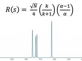
The primary relationships between resolution and column dimensions are outlined in Equation 1 and Table 1;

- Efficiency (N) is a function of - carrier gas type, column length (L), column internal diameter (dc)
- Retention Factor (k) is a function of - temperature, film thickness (df), column internal diameter (dc)
- Selectivity (α) is a function of – temperature (T), stationary phase chemistry
| Chromatographic Parameter | Length (L) | Internal Diameter (dc) | Film Thickness (df) |
| N | Increases | Increases with reducing diameter | - |
| k | - | Increases with reducing diameter | Increases with increasing film thickness |
| α | - | - | - |
Table 1: The relationship between chromatographic variable of the Resolution Equation and GC column dimensions.
So how can we relate the various GC column dimensions to resolution (Rs)? Combining Equation 1 with the information in Table 1 we can summarise the overall effects of column dimensions on chromatographic resolution using the following general relationships and caveats;
Column Length (L)
- Doubling column length doubles efficiency (N) which improves resolution by a factor of 1.4
- Doubles analysis time (or by approximately 1.5 – 1.75 times for gradient temperature programming)
- Increases column costs
- Need to consider the effects of elution temperature with increasing column length – may need to adjust oven temperature program
Column Internal Diameter (dc)
- Affects efficiency, retention, carrier flow rate, capacity and pressure drop across the column
- Column internal diameter is inversely proportional to column efficiency – halve column diameter, double efficiency, increase resolution by factor of 1.4
- Column head pressure is an inverse square function of column radius – so halving column diameter will increase head pressure (for an equivalent linear velocity) by a factor of 4
- Column capacity increases with column internal diameter, however capacity is also dependant on the stationary phase type, film thickness and the nature of the analytes
Stationary Phase Film Thickness (df)
- Affects retention, inertness, capacity, resolution and bleed
- Film thickness is directly proportional to retention time (or a ratio of 1.5:1 for gradient temperature programming)
- Thick stationary phase films give retention for highly volatile analytes
- Increasing film thickness allows retention of volatile analytes at temperatures at or above ambient
- Doubling stationary phase film thickness gives an increase of around 20oC in elution temperature
- Retention of late eluting (high boiling point) analytes is reduced using thinner film columns
- Early eluting analytes (k<2) are better resolved using thicker film columns
- Resolution may DECREASE for analytes with retention factor (k) values greater than around 5 with INCREASING film thickness
- Thicker films bleed more - upper temperature limits of thick film columns will be lower
- Thicker film columns are more inert as the film shields the analyte from active sites on the silica tubing (therefore better peak shape for polar and active compounds)
- Thicker film columns have higher analyte capacity, and so may reduce peak fronting
As always, it is better to visualise these effects using real life examples and so here we walk through some of the effects of changing GC column dimensions with the separation of Nitrosamine standards.
GC Conditions
| Column: | 5% phenyl polydimethylsiloxane (ultra-deactivated), 30.00 m, 0.25 mm ID, 0.25 µm |
| Carrier Gas: | Helium, Constant Flow @ 1.59 mL/min |
| Average Velocity: | 35.00 cm/sec |
| Outlet Pressure: | 14.70 psi (Atmospheric Pressure) |
| Oven Temp: | 40 °C (hold 5 min) to 80 °C @ 4 °C/min to 245 °C @ 8 °C/min |
Analytes
1.N-Nitrosodimethylamine, 2. N-Nitrosomethylethylamine, 3. N-Nitrosodiethylamine, 4. N-Nitrosopyrrolidine, 5. N-Nitrosomorpholine, 6. N-Nitrosodipropylamine, 7. N-Nitrosopiperidine, 8. N-Nitrosodibutylamine, 9. N-Nitrosodiethanolamine, 10. N-Nitrosodiphenylamine, 11. N-Nitrosonornicotine, 12. N-Nitrosodibenzylamine, 13. N-Nitrosonornicotine ketone
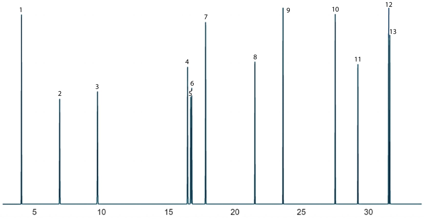
Figure 1: Separation of 13 different nitrosamine compounds using the conditions listed above.
From this separation we are particularly interested in optimising the separation of compounds 4 through 7 and will use the relationships described above to obtain an optimised separation for just these compounds of interest.
Figure 2 shows an expansion of the chromatogram to help us visualise the separation more clearly. In each of the separation optimisations, as we change the column dimensions, we will maintain a constant carrier gas linear velocity by adjusting the column head pressure to obtain 35cm/sec for the carrier gas (helium), unless otherwise stated.
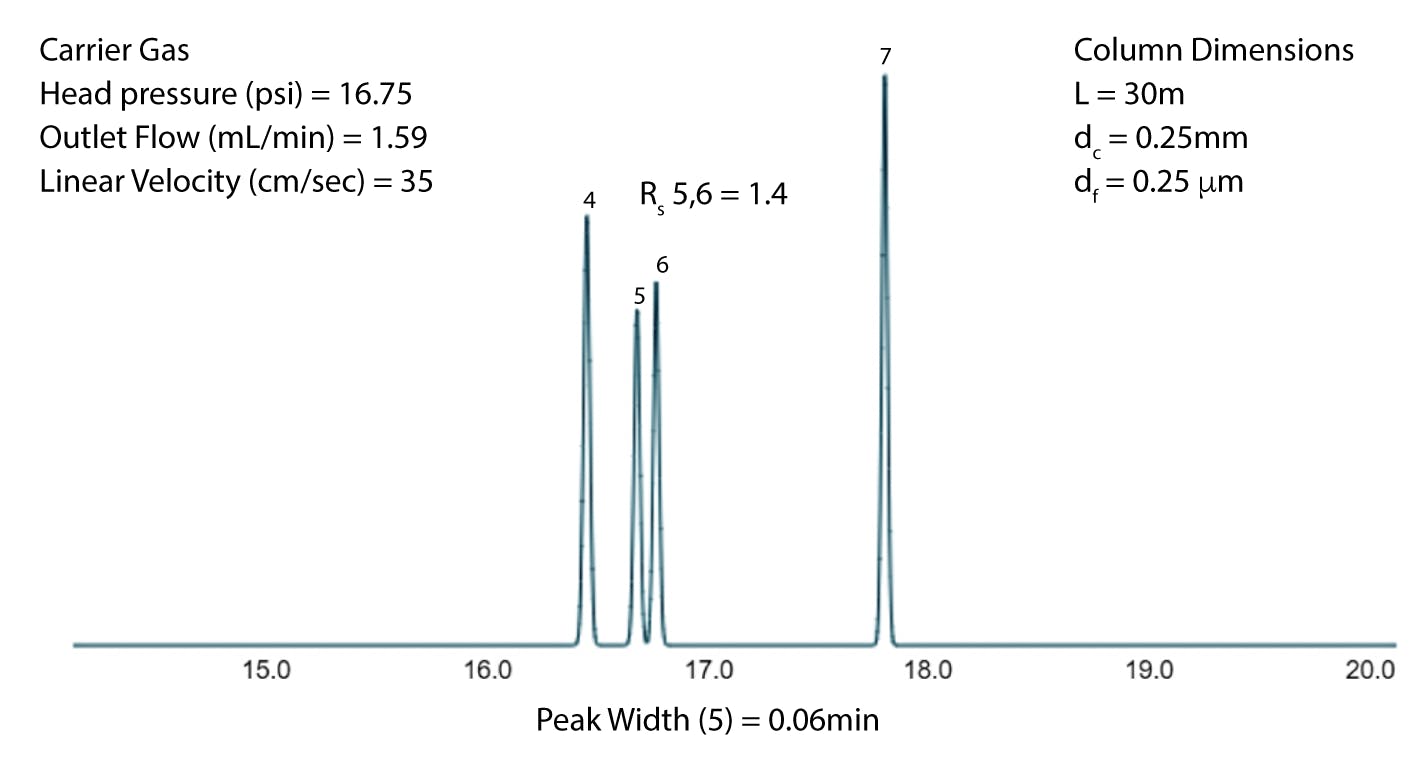
Figure 2: Expansion of chromatogram in Figure 1 to show key analytes of interest and the resolution between the critical peak pair.
At a resolution of 1.4, this method is going to be difficult to implement in practice and therefore we need to optimise the separation. Let’s see what happens when we change the column length to 15 and 60 meters to assess the effects.
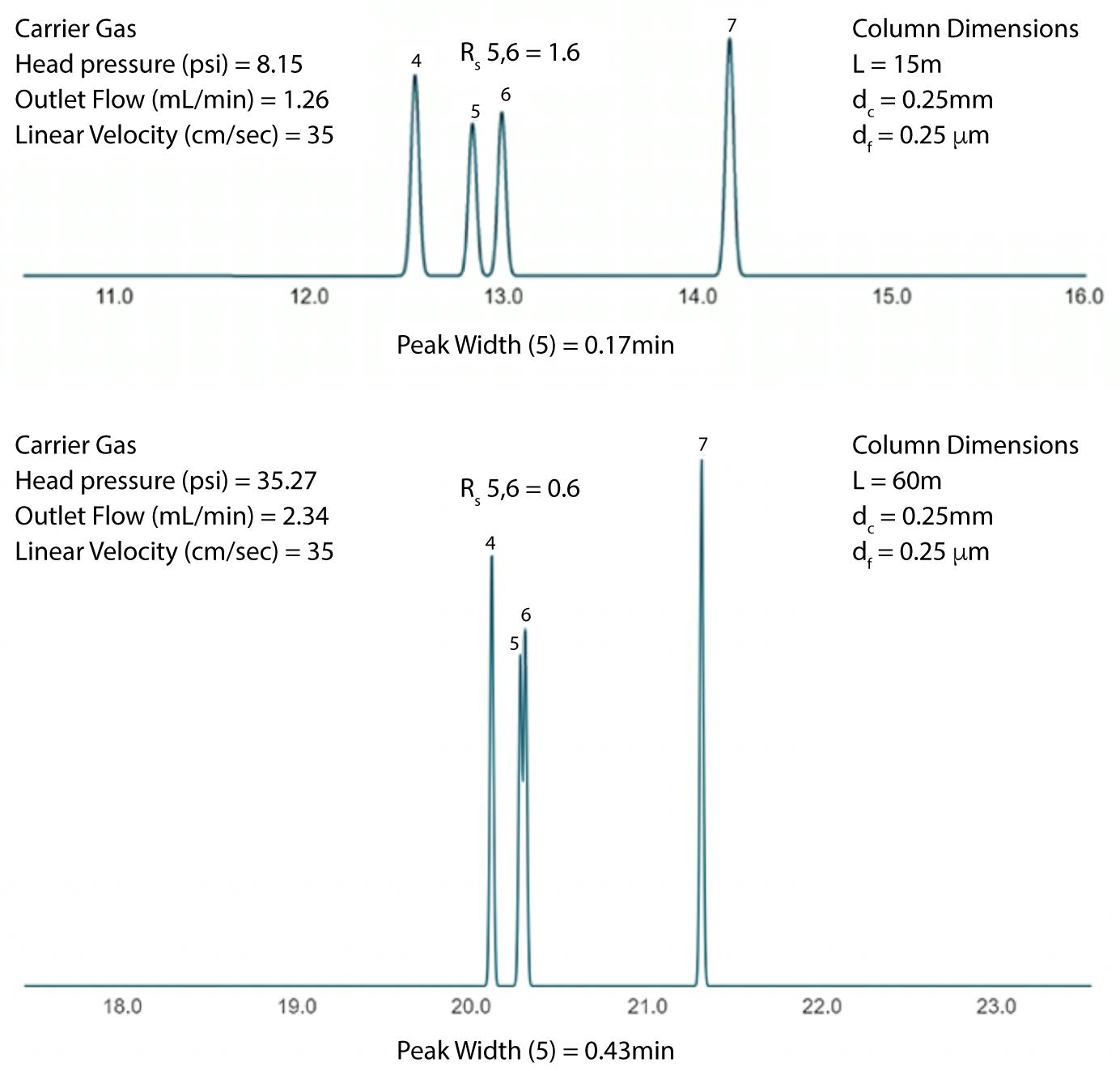
Figure 3: Expansion of chromatograms to show the analytes of interest using a 15m column (top) and 60m column (bottom), all other conditions are as per those in Figure 1 except the head pressure is adjusted to maintain a constant carrier gas linear velocity of 35 cm/sec.
Ouch! It would seem that as we increase column length, the resolution increase which was promised above, has not been realised! We can see that indeed the 15m column produces less efficiency (wider peak width at a constant linear velocity) and that the loner column delivers higher efficiency, again obvious from the decreased peak width when compared to the 30m column. So what has gone wrong?
Well, the eagle eyed amongst you will have noted the caveat that whilst longer columns deliver higher efficiency, we may also need to consider the oven temperature profile for this to offer improved resolution. If we were to calculate the actual elution temperature (i.e. the oven temperature at which the peak elutes from the GC column) for peak 5, for example, the results would be;
15m column = 71oC
30m column = 94oC
60m column = 122oC
We know from Equation 1, and the accompanying notes, that selectivity is influenced by changing column temperature, and so in order to optimise resolution when changing column length, we may also need to optimise the oven temperature program. The most practical way to do this is to use a program which enables translation of the oven temperature program (offered by most of the vendors of GC equipment), the results of which are shown in Figure 4.
GC Conditions
| Carrier Gas: | Helium, Constant Flow @ 1.59 mL/min |
| Average Velocity: | 35.00 cm/sec (30m) |
| Outlet Pressure: | 14.70 psi (Atmospheric Pressure) |
| Oven Temp: | 40 °C (hold 5 min) to 80 °C @ 4 °C/min to 245 °C @ 8 °C/min (30m column) 40 °C (hold 17 min) to 80 °C @ 1.2 °C/min to 245 °C @ 2.4 °C/min (60m column) |
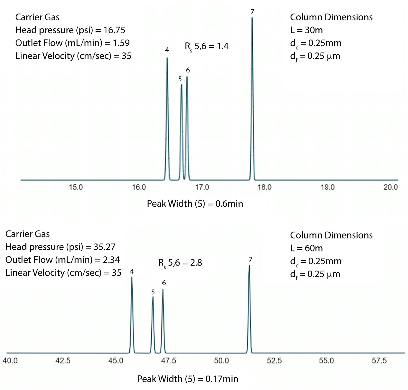
Figure 4: Comparison of chromatograms obtained from a 30m (top) and 60m (bottom) GC columns using translated oven temperature programs.
It will be obvious from Figure 4 that, by translating the oven temperature program, we have managed to significantly improve the resolution between the critical peak pair, and is certainly something we could comfortably work with on a routine basis. However, you will also have noticed that, alongside the new oven temperature program, we now have a much longer run time and that the chromatographic efficiency has significantly decreased (wider peaks than obtained with the original temperature program). However, for the huge increase in resolution we can live with the reduced efficiency and I’m sure the analysis time could have been shortened with a little experimentation.
Now let’s turn our attention to both column internal diameter and the effects of changing column i.d. on resolution. Figure 5 shows the results using a 30m column and internal diameters of 250 (original), 180 and 530mm. The original oven temperature program of Figure 1 was used in each case.
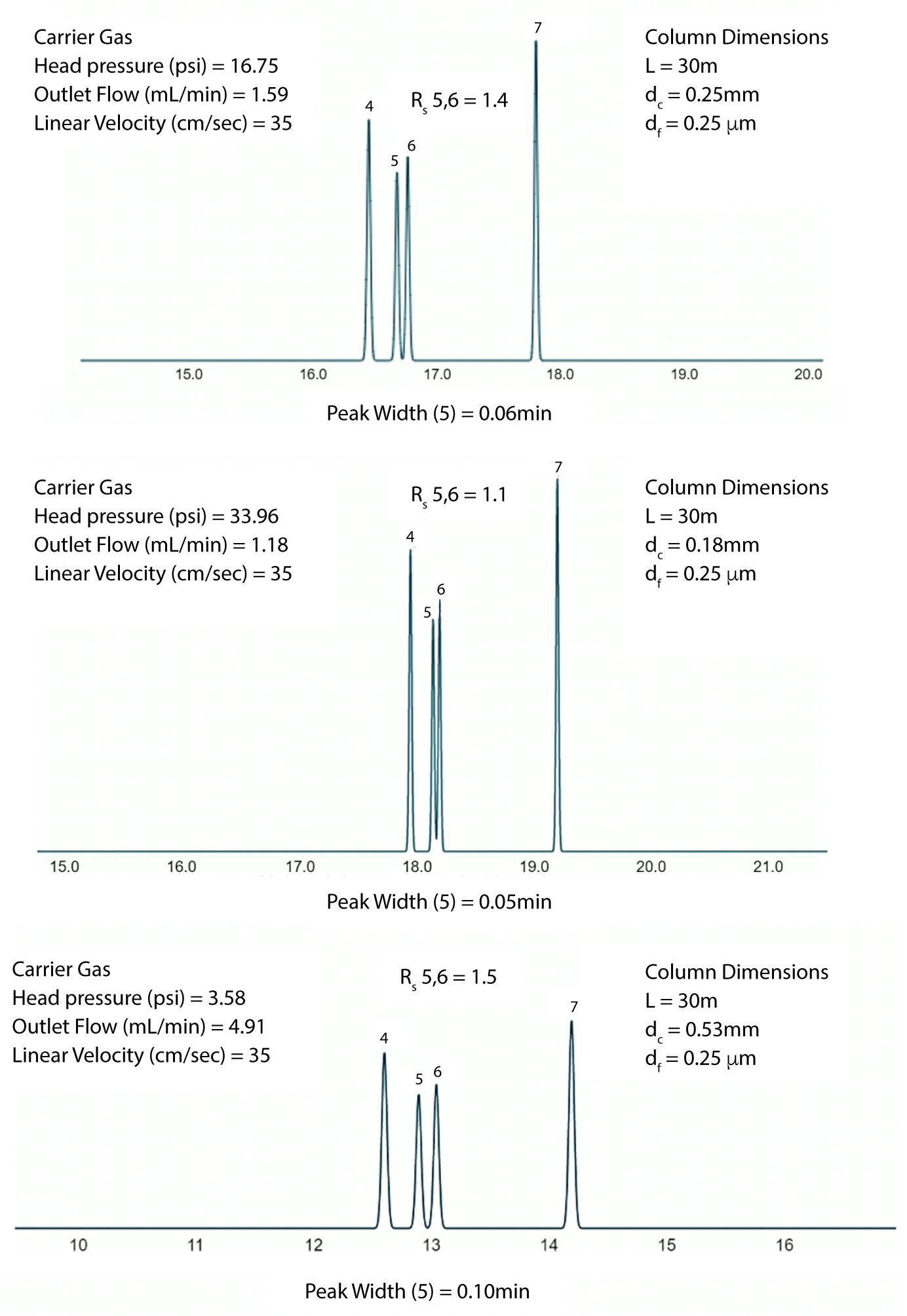
Figure 5: Comparison of chromatograms obtained from a 30m column with 0.25mm (top), 0.18mm (middle) and 0.53mm (bottom) internal diameter.
From Figure 5 we can see that we lose some resolution when the internal diameter is reduced and gain a little when it is increased (and the opposite effect is seen with efficiency or peak width). This makes sense of course, given that the k term increases when the internal dimeter is reduced, acting to reduce resolution and in this case we assume that the increase in k is greater than the increase in efficiency (N), thus resolution decreases with reducing internal diameter. Later we will look at a special case where when can overcome this.
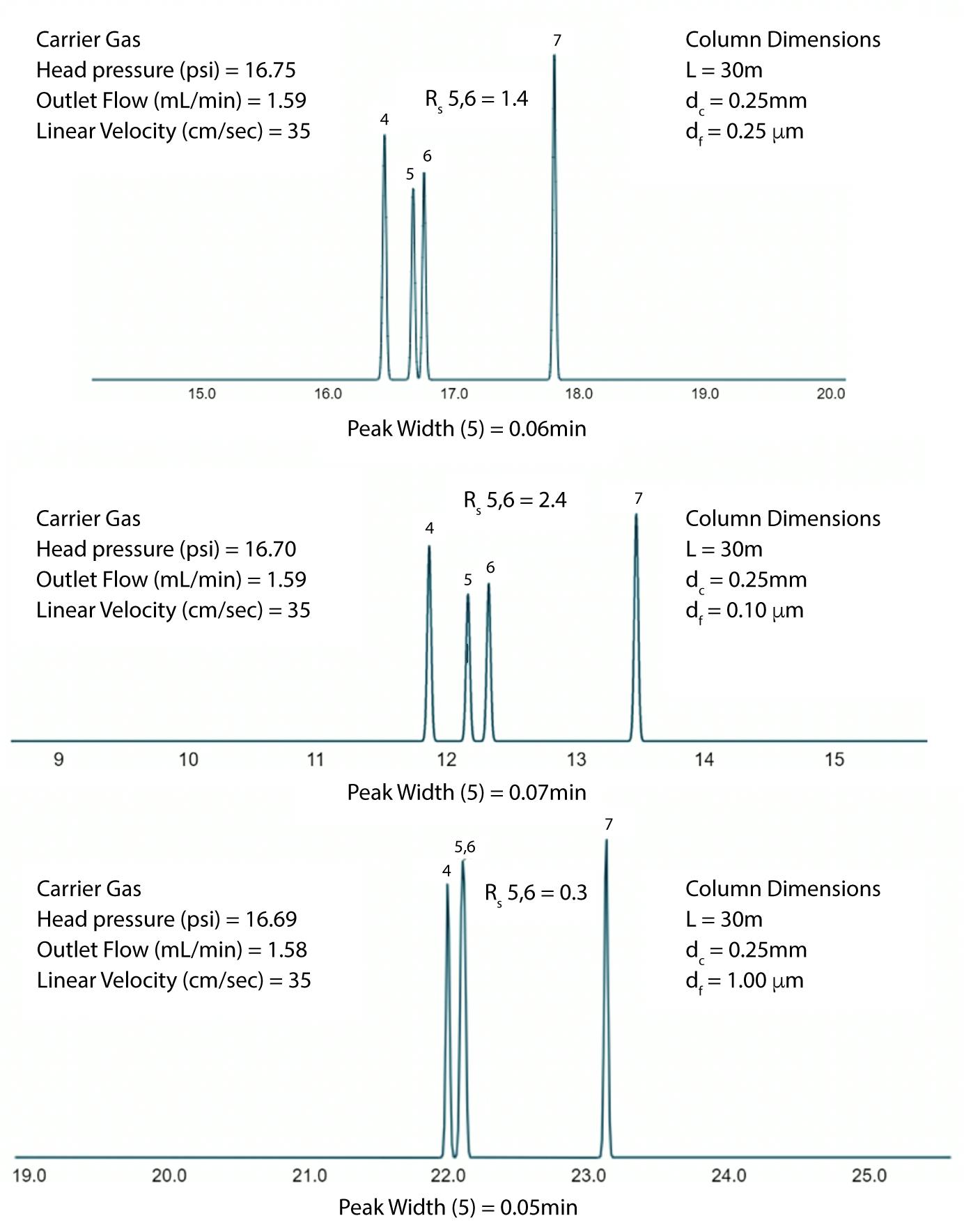
Figure 6: Comparison of chromatograms obtained from a 30m column with 0.25mm (top), 0.10mm (middle) and 1.00mm (bottom) film thickness.
From Figure 6 we can see that again the data follows our prediction and as we increase film thickness, retention factor increases and resolution decreases. What we also need to consider is that the column loadability (the amount of analyte we can load onto the column before peak shape begins to deform), is reduced by a factor of four when we move to the thinner film and increases by a factor of approximately 5 when we move to the thicker film. So, when making our stationary phase film thickness choice, we must always consider the column (stationary phase) loadability as well as the volatility of the analytes, and that more volatile analytes require thicker films for good retention.
To end, there is one reasonably special case that we should consider, and that is the combination of smaller internal diameter columns with relatively thin films. Here the effects of the increased retention are counterbalanced by the reduction in film thickness and we can often obtain very satisfactory separations. The added advantage is that to obtain a reasonable flow rate, column linear velocities are typically higher and therefore analysis tends to happen in shorter timeframes. This combination of smaller internal diameter with thinner films is often coined ‘fast GC’ as, not only are column flow rates higher, but shorter columns can often be used without any meaningful reduction of resolution.
Figure 7 shows an example of this in action. Note that the linear velocity has been optimised and the temperature program translated.
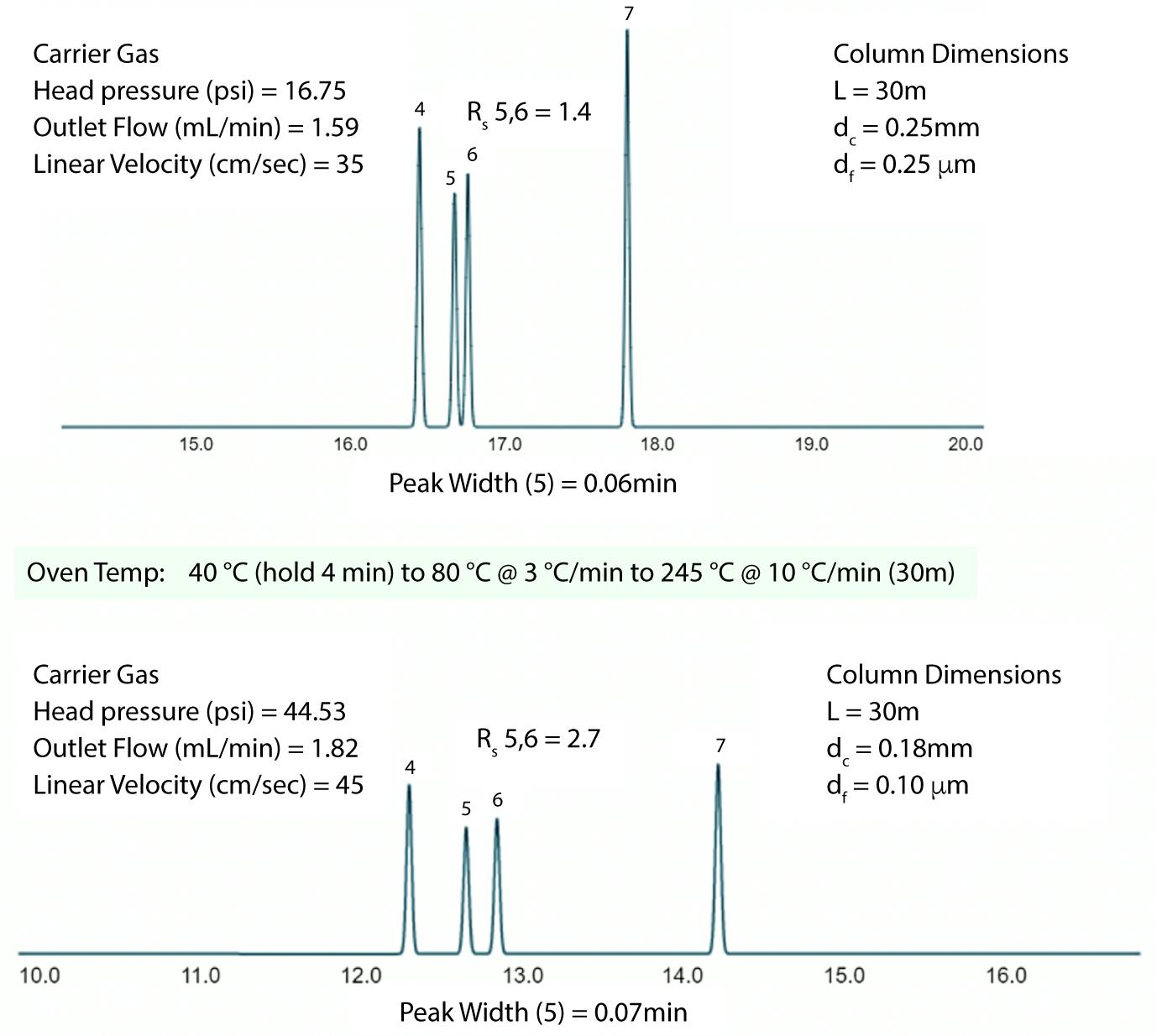
Figure 7: Comparison of chromatograms obtained from a 30m column with standard (top) and ‘reduced’ dimensions (bottom). Note that the linear velocity and oven temperature program have been further optimised in the bottom chromatogram.
From Figure 7 it should be immediately obvious that we are approaching the resolution obtained with the 60m column (Rs = 2.8), yet we have obtained this resolution in quarter of the analysis time – hence the power of what has become known as ‘Fast GC’. This would be a very acceptable set of conditions for routine analysis, provided that we do not load too much sample onto the column, which of course can be controlled by altering the inlet split ratio.
We have explored the basic relationships between column dimensions and resolution, considering the many caveats and rules of thumb which might guide our choices during method optimisation. Whilst it is not highly convenient to alter columns during the method development process, sometimes, if we run out of resolving power and cannot obtain a satisfactory separation by altering the oven temperature program, we have no choice but to alter either the stationary phase chemistry (and effectively start all over again!) or we can make some smart choices in altering the column dimensions to squeeze every last drop of resolution from our chromatographic system.
In writing this article I used some very useful tools which can help to model the separations that we may obtain and the translation of oven temperature and column flow conditions. I’ve listed links to these tools below;
Pro EZGC Chromatogram Modeler - Restek (Bellefonte, PA)
GC Method Translator - Agilent (Santa Clara, CA)
GC Calculators - Agilent (Santa Clara, CA)
Hopefully, you will carefully consider your choice of column dimension when planning and optimising your next separation!
Related articles