02 Dec 2020
Principal Component Analysis
The most rewarding part of our job at Element is to be able to help customers with their analytical problems. Sometimes that means recommending a different column, or a change in the method parameters. On other occasions we are asked to help with data processing and interpretation. This task can be complicated, especially when we deal with complex, multidimensional data sets.
Each object or observation in a multidimensional data set is described by a large number of attributes, variables, or dimensions. Examples could include pesticide multiresidue screening of soil samples, or nutritional and microbiological analysis of food products, where each sample can be described by dozens of variables. Data sets used in clinical research or metabolomics can include hundreds of dimensions.
Multivariate analysis is a general term that encompasses a number of techniques used to analyse multidimensional data. One of the most common multivariate tools is PCA, Principal Component Analysis. The most powerful advantage of PCA is that it can reduce the dimensions of the data set, from dozens of variables to only two or three, in order to facilitate visualisation and analysis.
This reduction cannot simply be done by culling variables, since we would lose the potentially valuable information contained in them. To reduce dimensionality whilst preserving as much information as possible, PCA transforms the data and presents it in a new set of dimensions, called Principal Components (PCs). Principal components are nothing more than linear combinations of the original variables, but they are calculated so that a small number of PCs encode as much of the original information as possible.
To illustrate the advantage of using PCA, we obtained a small data set from AAindex (https://www.genome.jp/aaindex/), a database of biochemical and physicochemical properties of amino acids. We tabulated 9 attributes for each amino acid: molecular weight, molecular weight of the peptide residue, pKa of the acidic group, pKb of the amino group, pK of the side chain, pI (isoelectric point), logP, logD at the isoelectric point, and polarizability.
Despite being a relatively small data set, it is difficult to grasp all the information at once. To begin with, the variables are measured in different units. Some have wide ranges of values, whilst others span a much narrower range. Some variables are strictly positive, while others have positive and negative values. This complexity makes it difficult to detect similarities, differences, or trends between amino acids.
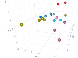
However, after applying PCA to the data, we were able to produce the following graph:
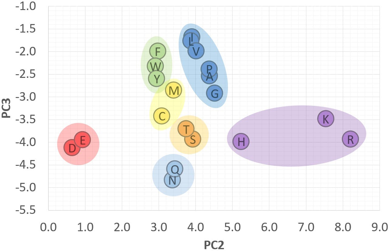
The nine multivariate dimensions were reduced to only three, PC1, PC2 and PC3, without any loss of information. In the new set of dimensions, the 20 amino acids appeared neatly clustered in the seven groups highlighted in the scatter plot. When we investigated the chemical properties of the amino acids searching for similarities, we realised that the seven groups corresponded to the following classification:
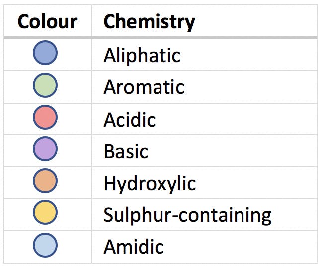
PCA gave us an insight into the data that was not obvious from the original variables. It is often said that PCA can reveal hidden patterns and connections between samples, as demonstrated in this example. This is an important and powerful characteristic of principal components, and a direct result of the way in which PCA highlights relationships between the original variables and uses these to better visualise the information contained in the data set.
A very simple example
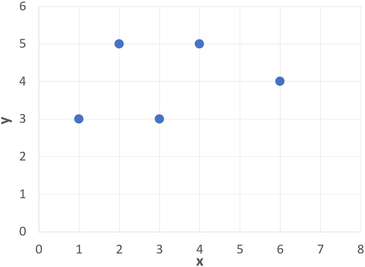
To illustrate how PCs work, let us imagine a number of data points such as these:
| x | y |
| 1 | 3 |
| 2 | 5 |
| 3 | 3 |
| 4 | 5 |
| 6 | 4 |
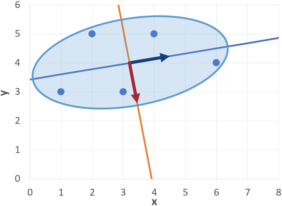
Note in the graph below that the cluster of points (blue dots) has a somewhat elongated, slanted profile:
If we try to draw an elliptical curve to enclose all the points, such as the blue area, we will find that:
- The optimum location for the centre of the ellipse is at the centroid of the cluster
- The axes of the ellipse (blue and orange diagonal lines) are tilted approximately 10 degrees counter-clockwise
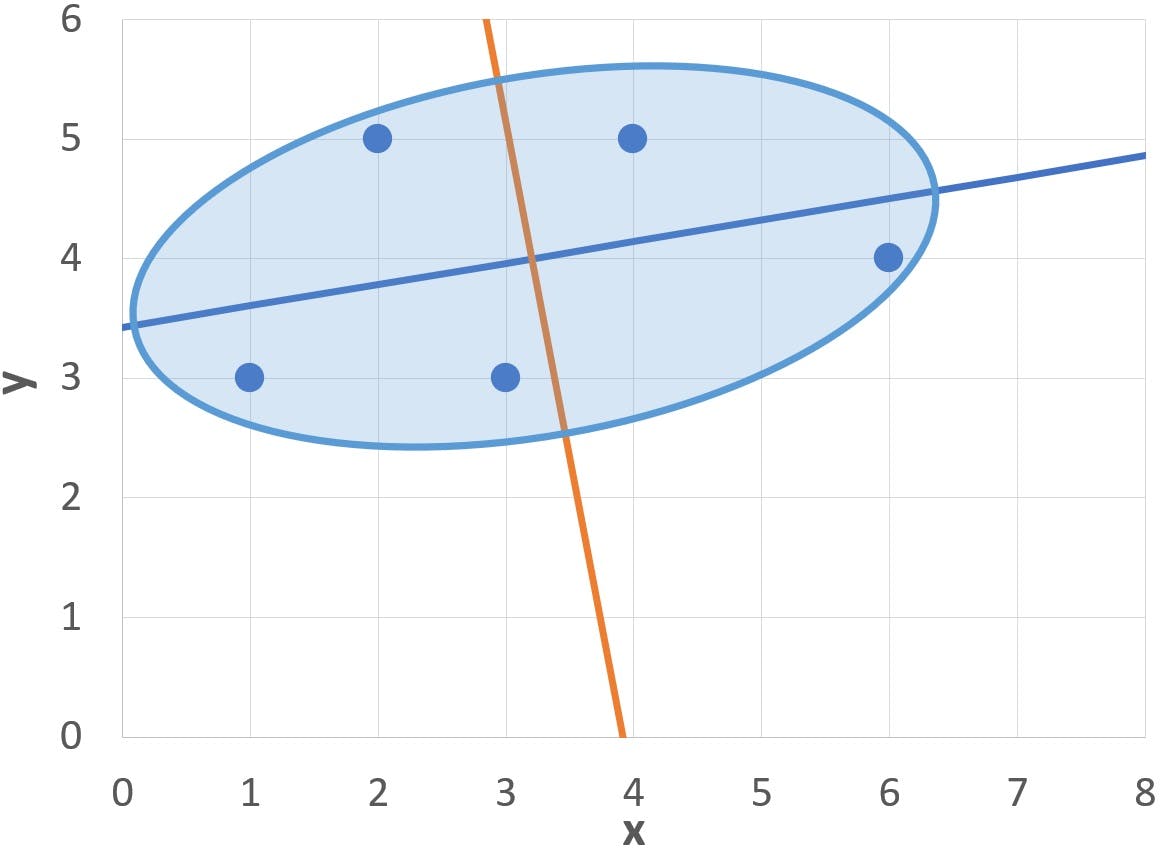
It turns out that the axes of the ellipse are, in fact, the two Principal Components of this particular cluster of points. And it is not too difficult to find them! The process of calculating the principal components has four stages:
- Calculate the covariance matrix of the original variables
- Extract the eigenvalues and eigenvectors of the covariance matrix
- Normalise each eigenvector to obtain the “loadings” of the original variables onto the PCs
- Calculate the “scores”, or coordinates of the data points on the PCs
Let’s do it step by step.
Covariance Matrix
First, calculate ![]() and
and ![]() , and subtract from the data points to obtain the “centred” data table. This will define the origin of the PCs:
, and subtract from the data points to obtain the “centred” data table. This will define the origin of the PCs:
 |
 |
| -2.2 | -1.0 |
| -1.2 | 1.0 |
| -0.2 | -1.0 |
| 0.8 | 1.0 |
| 2.8 | 0.0 |
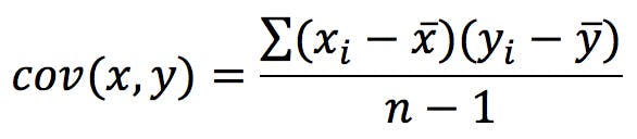
Second, calculate the covariance matrix, C. Covariance measures the extent to which two variables (x, y) increase in the same – or in opposite – directions. It is calculated with the following formula, the terms of which can be taken from the previous table:
Since we have two variables, x and y, the covariance matrix in our example will have four terms:
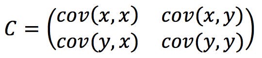
Note that cov (x, x) – the covariance of a variable with itself – is, by definition, the variance of the variable:
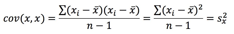
Also note that:
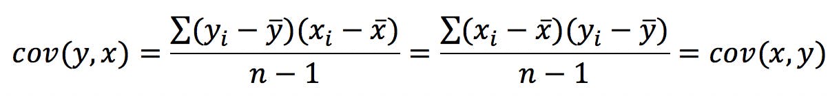
Hence the C matrix will always be symmetrical.
The calculations are as follows:
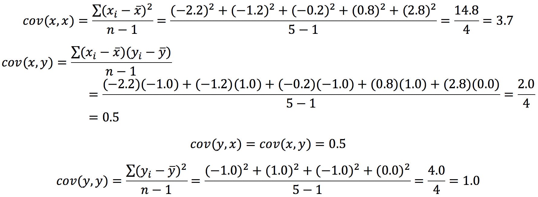
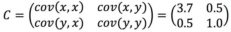
The resulting covariance matrix is:
Eigenvectors of the Covariance Matrix
It is obvious from the elongated shape of the cluster that the data points stretch further across the x axis than they do along the y axis: there is more “data variation” in the direction. The variance sx2(=3.7) is clearly higher than sy2(=1.0), which categorically confirms this. However, the cluster also appears to have some inclination: the direction of maximum variation is not horizontal, but slightly slanted.
The vectors (i.e. directions) of maximum and minimum variation of the data set are codified within the covariance matrix C. The next thing we need to do is “extract” these vectors, by solving the “eigenvectors equation”:
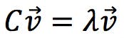
In algebra, matrices are used to represent linear transformations. The product of a matrix by a vector is equivalent to applying the linear transformation to the vector coefficients, resulting in a new vector with a different length or orientation. Eigenvectors are special cases: the linear transformation does not change their direction, it just changes their length by a scalar factor, λ. This factor is called the eigenvalue of that particular eigenvector.
The equation above can be expressed in this equivalent form:
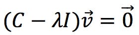
Where I is the identity matrix. This equation has a solution if and only if the following determinant is zero:
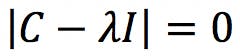
Developing this determinant results in the characteristic polynomial of the matrix C. For a 2×2 matrix of the form ![]() like our covariance matrix, the characteristic polynomial is:
like our covariance matrix, the characteristic polynomial is:
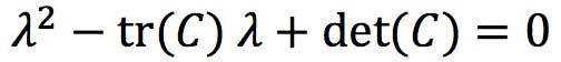
Where tr(C) = (a + d) is the trace, and det(C) = (ad - bc) is the determinant of C. The solutions of the polynomial, λ1 and λ2, are the eigenvalues of the matrix C.
In our example, tr(C) = 4.7, det(C) = 3.45 , therefore the solutions are:
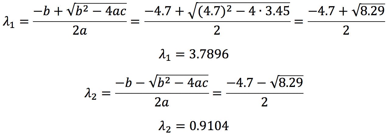
Solving the characteristic polynomial is the most complicated part of PCA. For 2×2 matrices, the polynomial is a quadratic equation that can be easily solved by the quadratic formula,
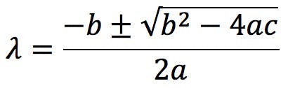
For an n×n matrix the characteristic polynomial is of degree n and, for most of us – certainly for me – solving polynomials of degree 3 or above really requires the use of a computer. Nevertheless, the complexity of the calculation should not detract from the fact that the underlying algebra is really simple and easy to understand.
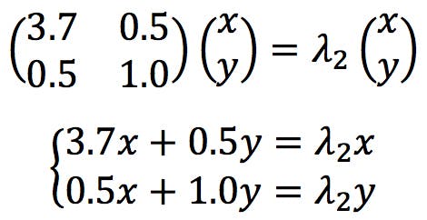
The next step in PCA is to calculate the eigenvector that corresponds to each eigenvalue. They are found by solving the following simultaneous equations
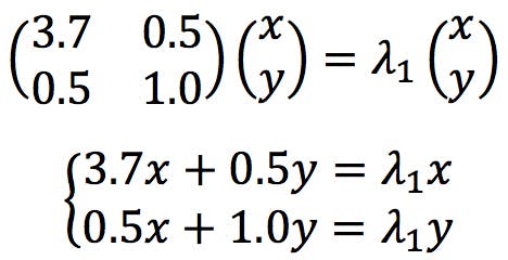
Developing the second equation:
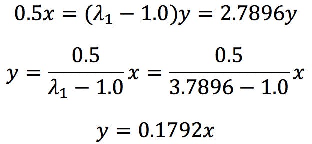
Applying to the first equation:

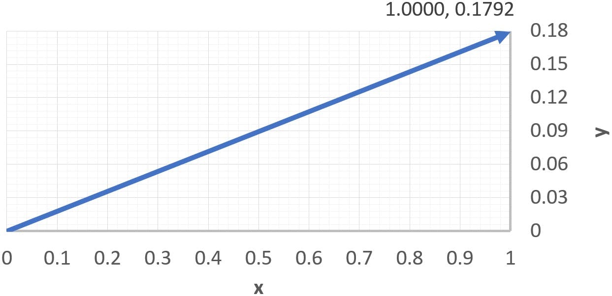
Therefore, x is independent and y = 0.1792x. The first eigenvector has the following coefficients:

The simultaneous equations for the second eigenvector would be solved in a similar way:
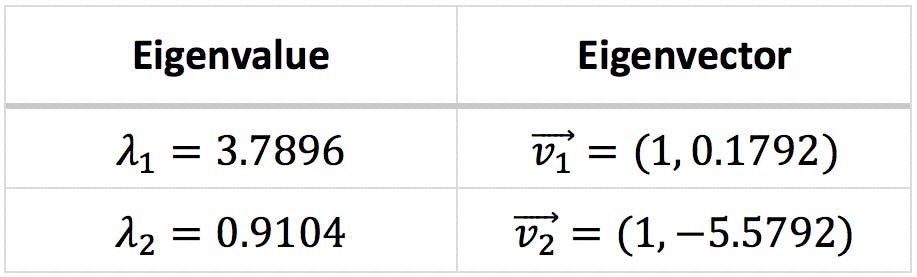
The resulting eigenvalues and eigenvectors are presented below:
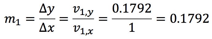
The following graph displays the first eigenvector as a dark blue arrow on the centre of the ellipse.
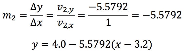
This is the generator vector for the major axis, in other words, the vector that defines the slope of the axis:
The major axis has the following equation:
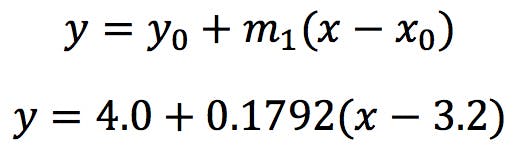
Where we have taken (x0, y0) = (3.2, 4.0) the centroid of the data set. As we hinted at earlier, this axis in not horizontal: it has a positive angle θ:

The second eigenvector (shown as a dark red arrow) generates the minor axis:
This axis is orthogonal to the major axis, with an angle of -79.84 degrees.
From a graphical point of view, PC1 and PC2 provide an alternative, optimised, set of axes on which to represent the data:
- The new origin is no longer but , the centroid of the data set.
- The new axes are no longer horizontal and vertical, but rather tilted 10.16 degrees counter-clockwise.
Loadings
So far, we know that PC1 is a linear combination of the original variables x and y. The contributions of the original variables onto the principal components are called “loadings”, because they indicate how much “weight” each one of them has on PC1 and PC2.
The first step to calculate the loadings is to normalise the eigenvectors, which consists in dividing them by their “length”, or norm. The norm of a vector is obtained by applying Pythagoras to its coefficients:

Thus, the normalised coefficients are:
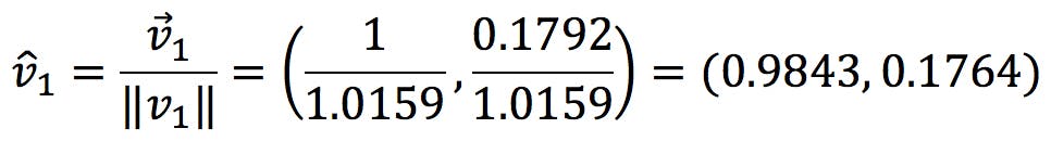
In other words,
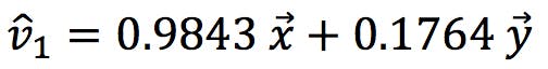
These normalised coefficients give us the “proportion” of x and y that make up the new variables: PC1 is 98.43% of x and 17.64% of y.
Similarly, for the second eigenvector, we find:
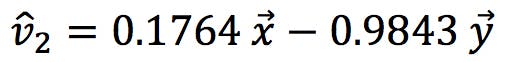
Therefore PC2 is 17.64% x and 98.43% - y (with a negative sign).
We can see that x has a large loading on PC1, but a much lower loading on PC2. By contrast, y has a low loading on PC1 but a large loading on PC2. This is very common: variables that have large contributions on one PC tend to have much lower loadings on the rest.
Scores
The final step in PCA is generally the graphical presentation the original data in the new frame of reference defined by the PCs. The coordinates of each object in the new system are called the “scores” of the object on PC1, PC2, etc. Calculating the scores is very simple: we just need to apply the normalised loadings found in the previous section to the (x, y) coordinates of the centred data points:
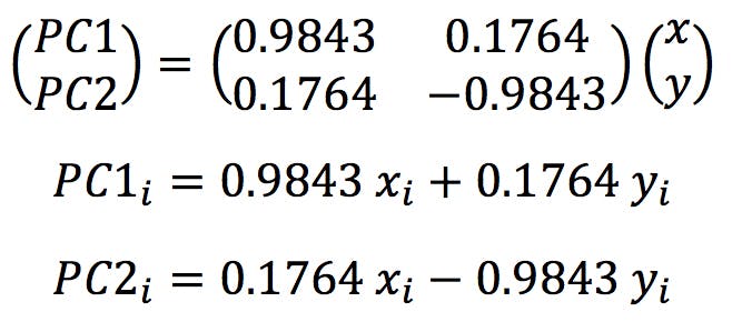
Where (xi, yi) are the original and (PC1i, PC2i) the new coordinates. The results are shown in the following table and plotted below:
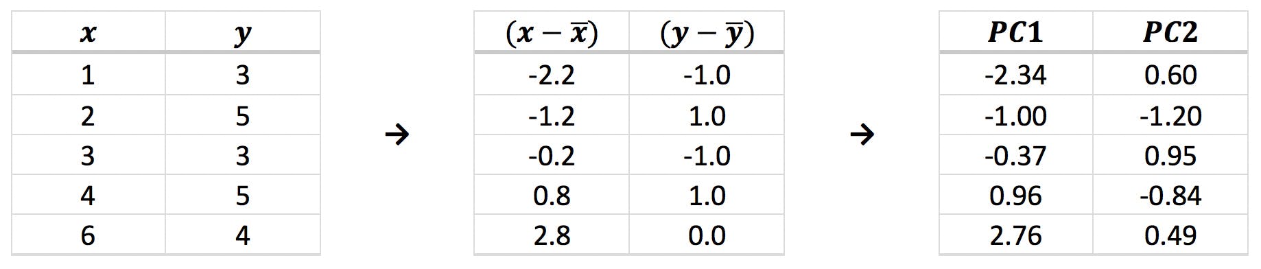
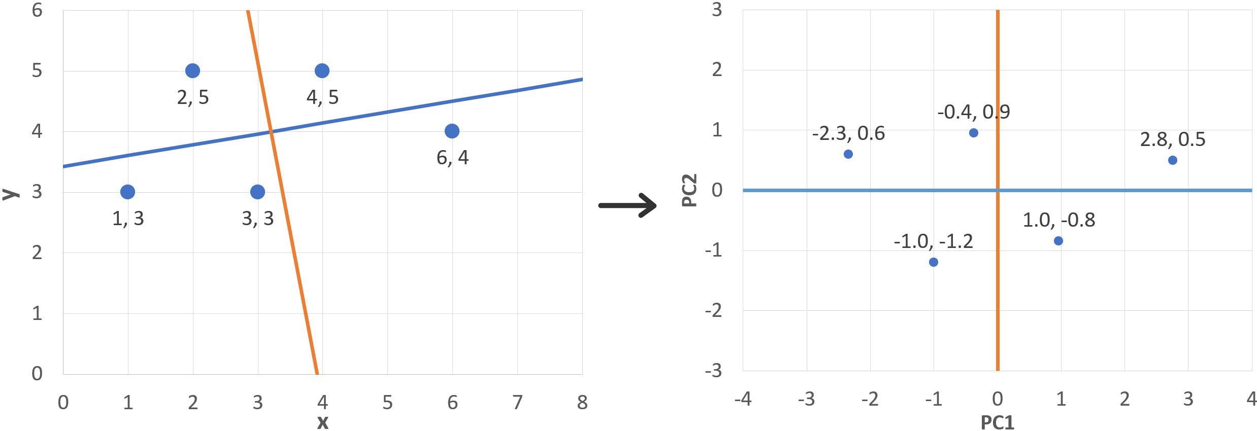
Notice that the points are centred around the origin, as expected, and slightly rotated compared to the original figure. This is the direct effect of the linear transformations effected by the eigenvectors. They are also “upside down”: remember that the second eigenvector (red arrow) points “down” (PC2i = 0.1764 xi - 0.9843 yi) and therefore inverts the y coordinates.
Eigenvalues and PC Variance
You will also notice that the first eigenvalue (λ1 = 3.7896) is around four times larger than the second one (λ2 = 0.9104). What is the significance of this?
Recall that the trace of the C matrix is the sum of the variances of x and y:
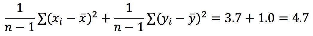
Interestingly, this is also the sum of the eigenvalues!

This is no coincidence: if eigenvectors generate these new variables called PCs, on which we can display our data points, we should be able to calculate data variance on each PC, S2PC1 and S2PC2, just as we calculate sx2 and sy2. It turns out that each eigenvalue gives us the data variance over its corresponding eigenvector:
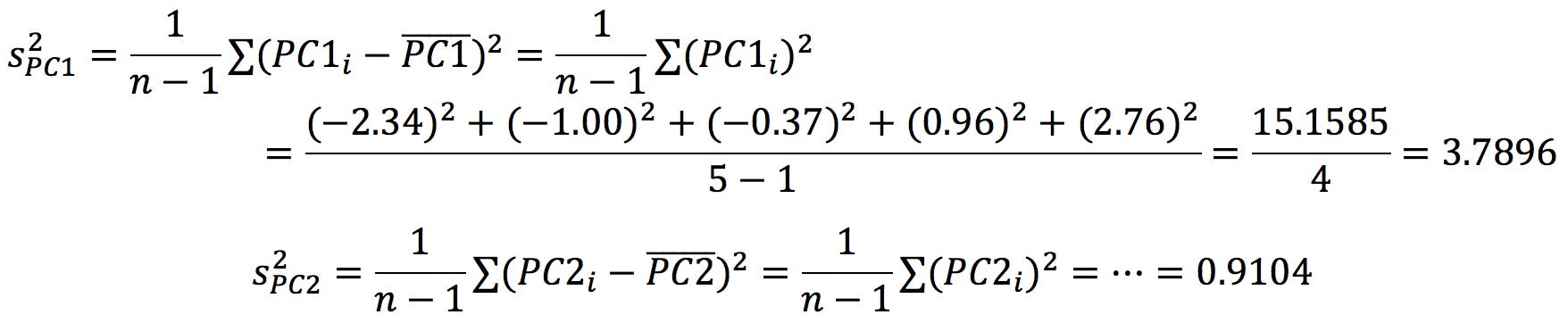
where I have simplified the equations because ![]() =
= ![]() = 0. The variance over PC1 is, therefore, 80.6% of the total variance. In other words, PC1 “encodes” 80.6% of the information:
= 0. The variance over PC1 is, therefore, 80.6% of the total variance. In other words, PC1 “encodes” 80.6% of the information:
| Eigenvalue | Variance | Percentage |
| λ1 | 3.7896 | 80.6% |
| λ2 | 0.9104 | 19.4% |
| Total | 4.7000 | 100.0% |
Reducing Data Set Dimensions
I started this discussion explaining that principal components are used to reduce the dimensionality of large data sets. So far, I have only shown that they provide an alternative system of coordinates. However, we have also seen that 80.6% of data variation occurs along the PC1 axis.
If we wanted to reduce this data set to a single dimension, while still preserving the maximum amount of information, the optimum course of action would be to project the five data points onto PC1. The projections are shown in the following graph as yellow points:
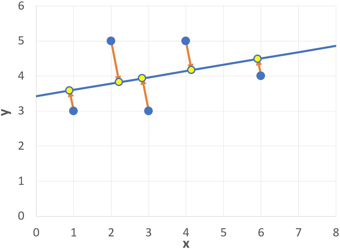
Of course, the projections give no information about how far above or below the axis the original dots were positioned: this is the 19.4% of information accounted for by the second PC.
Learning Points
This simple example illustrates several characteristics of principal components:
- A principal component (PC) is a linear combination of the original variables.
- PCs can be visualised as alternative axes on which to represent the data.
- Each PC is generated by an eigenvector of the data covariance matrix.
- A data set with k variables has a k x k covariance matrix, with keigenvectors and, therefore, k PCs.
- Eigenvectors are orthogonal to each other, and so are the generated PCs.
- Each eigenvector has a corresponding eigenvalue (λ) that indicates the amount of variance explained by the PC.
- Eigenvectors are often ranked from highest to lowest λ, so that the first PC (PC1) explains the largest fraction of data variance; the second PC explains (the largest part of) the variance not encoded by PC1, PC3 explains the variance not explained by PC2, etc.
- The first few PCs (PC1, PC2, PC3…) can often be successfully used to reduce the dimensionality of a multidimensional data set, in order to facilitate visualisation and analysis whilst minimising the loss of information.
Conclusions
Principal Component Analysis is utilised in countless applications, from image processing to social sciences, financial analysis, or proteomics research. Whenever complex data sets need to be compacted or simplified for further analysis, PCA has a role to play. Despite its widespread use, PCA is still not well understood by many of us, not least because the calculations involved are nigh impossible. I wouldn’t expect anybody to calculate principal components by hand, but I hope this worked example will help visualise the steps involved and clarify some of the mysteries surrounding PCA.
In a future instalment, I will address some larger data sets to explore other interesting properties of Principal Components. I gladly welcome comments and questions, and if you have a specific topic you would like us to discuss, please don’t hesitate to get in touch.
Related articles