01 Feb 2021
Principal Component Analysis part 2
In a previous instalment of this blog, we covered the “ABC” of PCA (Principal Component Analysis) by examining how this method would be applied to a very simple example: five points on a plane:


As described in that article, principal components (PCs) are a new set of variables obtained from a combination of the original variables. The steps involved in PCA are the following:
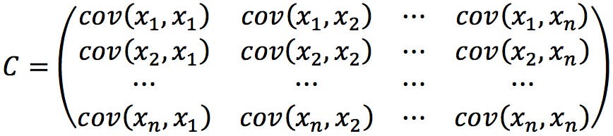
- Calculate the covariance matrix, C, of the data set
- Extract the eigenvalues (λ) and eigenvectors (
 ) of the covariance matrix
 - Normalise eigenvectors to calculate the loadings (coefficients) of the original variables onto each principal component
- Calculate the scores (coordinates) of the original data points in the new PC space
A multivariate data set containing n variables can be thought of as a scatter of points in an n-dimensional space. Unfortunately, if the number of variables is greater than three, there is no easy way to visualise these points. The matrix C is an (n x n) matrix (i.e. a matrix of rank n) of the covariances measured between each pair of variables. Any matrix of rank n can be described by an arbitrary set of n orthogonal vectors, called basis vectors. One particular set of basis vectors of the C matrix, called ‘eigenvectors’ of C, describe the directions in which the data set points are spread or scattered.
Each eigenvector has an associated eigenvalue, a number which corresponds to the data variance measured along the direction of the eigenvector. The eigenvector with the largest eigenvalue, therefore, points in the direction of maximum spread. The eigenvector with the second largest eigenvalue indicates the direction of second highest scatter, etc. These orthogonal eigenvectors define the new axes PC1, PC2, …, PCn. Consequently, the first PC axis has been constructed so that it describes as much of the variance in the data set as possible, and successive PCs describe increasingly smaller proportions of variance.
The advantage of representing the data points in this new set of axes is that, in many cases, it is possible to simplify an abstract multidimensional space down to two or three easy to visualise dimensions. By creating a scatter plot of PC1, PC2 and PC3 – the directions of maximum variance – the simplified graph will still be able to convey a large amount of the information contained in the multidimensional space.
A Slightly More Complex Data Set
AAindex is an impressive repository of amino acid data compiled from hundreds of peer-reviewed papers, and it is a good source of data to learn multivariate analysis. To describe more advanced aspects of PCA, I decided to use the following set of variables from AAindex:
Table 1:Selected numerical descriptors of proteinogenic amino acids.
| Name | Abbr. | Symbol | MW | Residue MW (-H2O) |
pKa | pKb | pKx | pl | logD (pI) | Polarisability | Normalised Volume |
| Alanine | Ala | A | 89.10 | 71.08 | 2.34 | 9.69 | 6.00 | -2.841 | 8.478 | 1.00 | |
| Arginine | Arg | R | 174.20 | 156.19 | 1.82 | 8.99 | 12.48 | 10.76 | -3.156 | 18.035 | 6.13 |
| Asparagine | Asn | N | 132.12 | 114.11 | 2.02 | 8.80 | 5.41 | -4.288 | 11.810 | 2.95 | |
| Aspartic acid | Asp | D | 133.11 | 115.09 | 1.88 | 9.60 | 3.65 | 2.77 | -3.504 | 11.418 | 2.78 |
| Cysteine | Cys | C | 121.16 | 103.15 | 1.92 | 8.35 | 8.18 | 5.05 | -2.792 | 11.482 | 2.43 |
| Glutamic acid | Glu | E | 147.13 | 129.12 | 2.10 | 9.67 | 4.25 | 3.22 | -3.241 | 13.488 | 3.78 |
| Glutamine | Gln | Q | 146.15 | 128.13 | 2.17 | 9.13 | 5.65 | -4.001 | 13.866 | 3.95 | |
| Glycine | Gly | G | 75.07 | 57.05 | 2.35 | 9.78 | 5.97 | -3.409 | 6.636 | 0.00 | |
| Histidine | His | H | 155.16 | 137.14 | 1.82 | 9.17 | 6.00 | 7.59 | -3.293 | 14.926 | 4.66 |
| Isoleucine | Ile | I | 131.18 | 113.16 | 2.36 | 9.68 | 6.02 | -1.508 | 14.268 | 4.00 | |
| Leucine | Leu | L | 131.18 | 113.16 | 2.36 | 9.60 | 5.98 | -1.586 | 14.325 | 4.00 | |
| Lysine | Lys | K | 146.19 | 128.18 | 2.16 | 9.18 | 10.53 | 9.74 | -3.215 | 16.009 | 4.77 |
| Methionine | Met | M | 149.21 | 131.20 | 2.28 | 9.21 | 5.74 | -2.189 | 15.529 | 4.43 | |
| Phenylalanine | Phe | F | 165.19 | 147.18 | 2.16 | 9.18 | 5.48 | -1.184 | 17.197 | 5.89 | |
| Proline | Pro | P | 115.13 | 97.12 | 1.95 | 10.64 | 6.30 | -2.569 | 11.469 | 2.72 | |
| Serine | Ser | S | 105.09 | 87.08 | 2.19 | 9.21 | 5.68 | -3.888 | 9.448 | 1.60 | |
| Threonine | Thr | T | 119.12 | 101.11 | 2.09 | 9.10 | 5.66 | -3.471 | 11.008 | 2.60 | |
| Tryptophan | Trp | W | 204.23 | 186.22 | 2.43 | 9.44 | 5.89 | -1.085 | 21.197 | 8.08 | |
| Tyrosine | Tyr | Y | 181.19 | 163.18 | 2.20 | 9.11 | 10.07 | 5.66 | -1.489 | 18.204 | 6.47 |
| Valine | Val | V | 117.15 | 99.13 | 2.32 | 9.62 | 5.96 | -1.953 | 12.238 | 3.00 |
In this table,
- MW is the molecular weight of the amino acid
- Residue MW is the molecular weight after peptide condensation (after loss of H2O)
- pKa, pKb and pKx refer to the acidic (C-terminus), basic (N-terminus) and side chain (where applicable)
- pI is the isoelectric point of the amino acid
- logD (pI) is the distribution coefficient measured at the isoelectric point
- Polarisability is related to the dipole moment of the amino acid
- Normalised Volume refers to the bulkiness of the side chain, with glycine (side chain: -H) having an arbitrary value of zero
Dealing with Missing Data
If we try to calculate PCA on this data using a statistics package, we are likely to get an error. This is caused by the missing values in the pKx column, which prevent us from calculating the covariance matrix:
Where:
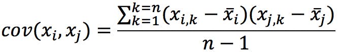
If any of the x i,k values are missing, the programme will not know how to calculate the covariance matrix. To resolve the problem, we can simply eliminate the variable form the database. Alternatively, if we believe that the information is critical to the analysis, we can try to “pad” the missing values. A quick look at a pKa table shows that pKa values for alcohols are typically estimated to be above 15, above 20 for amides, and above 40 for hydrocarbons. We could therefore fill the blanks with a constant value (e.g. 20) to indicate that these species have neutral side chains.
After padding the missing data points, the resulting covariance matrix is:
Table 2: Covariance matrix of nine selected variables, corrected for missing values.
| MW | Residue MW (-H2O) |
pKa | pKb | pKx | pl | logD (pI) | Polarisability | Normalised Volume |
|
| MW | 952.538 | 952.599 | -0.706 | -4.285 | -51.409 | 11.138 | 12.881 | 106.491 | 58.566 |
| Residue MW (-H2O) |
952.599 | 952.661 | -0.706 | -4.286 | -51.411 | 11.139 | 12.881 | 106.497 | 58.569 |
| pKa | -0.706 | -0.706 | 0.037 | 0.024 | 0.742 | -0.048 | 0.094 | 0.010 | -0.003 |
| pKb | -4.285 | -4.286 | 0.024 | 0.216 | 0.660 | -0.121 | 0.096 | -0.384 | -0.199 |
| pKx | -51.409 | -51.411 | 0.742 | 0.660 | 38.739 | 1.051 | 1.291 | -3.267 | -1.858 |
| pI | 11.138 | 11.139 | -0.048 | -0.121 | 1.051 | 3.130 | -0.015 | 2.087 | 1.027 |
| logD (pI) | 12.881 | 12.881 | 0.094 | 0.096 | 1.291 | -0.015 | 0.967 | 1.979 | 1.053 |
| Polarisability | 106.491 | 106.497 | 0.010 | -0.384 | -3.267 | 2.087 | 1.979 | 12.702 | 6.880 |
| Normalised Volume |
58.566 | 58.569 | -0.003 | -0.199 | -1.858 | 1.027 | 1.053 | 6.880 | 3.758 |
Highly Correlated Variables
Remember from the first instalment that the elements in the diagonal are the variances of the variables:
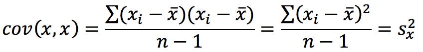
It is very clear that the first two variables (MW and Residue MW) have much larger variances than the rest. We can predict that the first principal component will have very large loadings on these two variables, whereas the rest will mostly contribute to higher order PCs.
Notice also the very high covariance (952.599) between MW and Residue MW. What does this mean? Calculating the correlation between MW and Residue MW results in an : from an information perspective, the two variables are essentially identical and one of them could be safely removed without any loss in data quality.
We confirm these predictions after carrying out PCA and observing the eigenvalues and loadings (only the first four PCs are shown for brevity):
Table 3: Eigenvalues of PCA on nine selected variables.
| Eigenvalue | λ | % of Total |
| 1 | 1923.84 | 97.92% |
| 2 | 36.38 | 1.85% |
| 3 | 3.16 | 0.16% |
| 4 | 1.11 | 0.06% |
Table 4: Loadings of first four principal components.
| Variable | Loading PC1 | Loading PC2 | Loading PC3 | Loading PC4 |
| MW | 0.704 | 0.021 | -0.025 | 0.044 |
| Residue MW | 0.704 | 0.021 | -0.025 | 0.045 |
| pKa | -0.001 | 0.020 | -0.021 | -0.078 |
| pKb | -0.003 | 0.012 | -0.025 | -0.172 |
| pKx | -0.039 | 0.993 | -0.068 | 0.089 |
| pI | 0.008 | 0.051 | 0.954 | 0.137 |
| logD (pI) | 0.010 | 0.057 | -0.055 | -0.757 |
| Polarisability | 0.079 | 0.074 | 0.264 | -0.550 |
| Norm Volume | 0.043 | 0.039 | 0.101 | -0.241 |
Recall from the first instalment that each eigenvalue indicates the variance over the corresponding principal component. Table 3 shows that PC1 accounts for nearly 98% of the variation, whereas the rest of PCs only make marginal contributions to the description of the data set.
Table 4, on the other hand, shows the loadings of the original variables on the first few PCs. It is clear that PC1 receives the greatest contributions from MW and Residual MW, whereas the effects of the other variables on this PC are at least an order of magnitude smaller. On the other hand, it is interesting to note that the loadings of MW and Residual MW are practically identical on all principal components: the two variables contribute in the same way to the new dimensions. Since the main objective of PCA is the reduction of data dimensionality, it is clear that we can afford to make one of these variables redundant, simplifying the data set without loss of information. Further analysis will be carried out on just eight of the variables:
Table 5: Eight selected variables for further PCA.
| Name | Abbr. | Symbol | MW | pKa | pKb | pKx | pl | logD | Polar | NV |
| Alanine | Ala | A | 89.10 | 2.34 | 9.69 | 20.00 | 6.00 | -2.841 | 8.478 | 1.00 |
| Arginine | Arg | R | 174.20 | 1.82 | 8.99 | 12.48 | 10.76 | -3.156 | 18.035 | 6.13 |
| Asparagine | Asn | N | 132.12 | 2.02 | 8.80 | 20.00 | 5.41 | -4.288 | 11.810 | 2.95 |
| Aspartic acid | Asp | D | 133.11 | 1.88 | 9.60 | 3.65 | 2.77 | -3.504 | 11.418 | 2.78 |
| Cysteine | Cys | C | 121.16 | 1.92 | 8.35 | 8.18 | 5.05 | -2.792 | 11.482 | 2.43 |
| Glutamic acid | Glu | E | 147.13 | 2.10 | 9.67 | 4.25 | 3.22 | -3.241 | 13.488 | 3.78 |
| Glutamine | Gln | Q | 146.15 | 2.17 | 9.13 | 20.00 | 5.65 | -4.001 | 13.866 | 3.95 |
| Glycine | Gly | G | 75.07 | 2.35 | 9.78 | 20.00 | 5.97 | -3.409 | 6.636 | 0.00 |
| Histidine | His | H | 155.16 | 1.82 | 9.17 | 6.00 | 7.59 | -3.293 | 14.926 | 4.66 |
| Isoleucine | Ile | I | 131.18 | 2.36 | 9.68 | 20.00 | 6.02 | -1.508 | 14.268 | 4.00 |
| Leucine | Leu | L | 131.18 | 2.36 | 9.60 | 20.00 | 5.98 | -1.586 | 14.325 | 4.00 |
| Lysine | Lys | K | 146.19 | 2.16 | 9.18 | 10.53 | 9.74 | -3.215 | 16.009 | 4.77 |
| Methionine | Met | M | 149.21 | 2.28 | 9.21 | 20.00 | 5.74 | -2.189 | 15.529 | 4.43 |
| Phenylalanine | Phe | F | 165.19 | 2.16 | 9.18 | 20.00 | 5.48 | -1.184 | 17.197 | 5.89 |
| Proline | Pro | P | 115.13 | 1.95 | 10.64 | 20.00 | 6.30 | -2.569 | 11.469 | 2.72 |
| Serine | Ser | S | 105.09 | 2.19 | 9.21 | 20.00 | 5.68 | -3.888 | 9.448 | 1.60 |
| Threonine | Thr | T | 119.12 | 2.09 | 9.10 | 20.00 | 5.66 | -3.471 | 11.008 | 2.60 |
| Tryptophan | Trp | W | 204.23 | 2.43 | 9.44 | 20.00 | 5.89 | -1.085 | 21.197 | 8.08 |
| Tyrosine | Tyr | Y | 181.19 | 2.20 | 9.11 | 10.07 | 5.66 | -1.489 | 18.204 | 6.47 |
| Valine | Val | V | 117.15 | 2.32 | 9.62 | 20.00 | 5.96 | -1.953 | 12.238 | 3.00 |
Step by Step Principal Component Analysis
In my previous instalment, I started PCA by subtracting the averages of the original variables from each data point, to obtain a table of centred values. This transformation is convenient when doing manual calculations, but it is not universally performed by statistical software. For the remainder of this article I will use Minitab 16, which does not centre the variables. If I wished to do so, I should select the command ‘Standardize’ from the ‘Calc’ menu, and select the option ‘Subtract mean’. Alternatively, the data could be transformed in a spreadsheet and copied into the software.
Covariance Matrix
The covariance calculated on the eight variables in Table 5 is displayed below. After dispensing with Residue MW, the rest of covariances remain the same as Table 2. MW still has a very high variance and we expect this variable to weigh heavily on PC1.
Table 6: Covariance matrix of the eight selected variables.
| MW | pKa | pKb | pKx | pl | logD | Polar | NV | |
| MW | 952.538 | -0.706 | -4.285 | -51.409 | 11.138 | 12.881 | 106.491 | 58.566 |
| pKa | -0.706 | 0.037 | 0.024 | 0.742 | -0.048 | 0.094 | 0.010 | -0.003 |
| pKb | -4.285 | 0.024 | 0.216 | 0.661 | -0.121 | 0.096 | -0.384 | -0.199 |
| pKx | -51.409 | 0.742 | 0.660 | 38.739 | 1.051 | 1.291 | -3.267 | -1.858 |
| pl | 11.138 | -0.048 | -0.121 | 1.051 | 3.130 | -0.015 | 2.087 | 1.027 |
| logD | 12.881 | 0.094 | 0.096 | 1.291 | -0.015 | 0.967 | 1.979 | 1.053 |
| Polar | 106.491 | 0.010 | -0.384 | -3.268 | 2.087 | 1.979 | 12.702 | 6.880 |
| NV | 58.566 | -0.003 | -0.199 | -1.858 | 1.027 | 1.053 | 6.880 | 3.758 |
Eigenvectors of the Covariance Matrix and Scree Test
The eight eigenvectors of Table 6 are displayed below:
| Eigenvalue | λ | % |
| 1 | 971.225 | 95.96% |
| 2 | 36.344 | 3.59% |
| 3 | 3.159 | 0.31% |
| 4 | 1.105 | 0.11% |
| 5 | 0.164 | 0.02% |
| 6 | 0.071 | 0.01% |
| 7 | 0.013 | 0.00% |
| 8 | 0.007 | 0.00% |
The variance ascribed to the first PC has dropped somewhat, but PC1 still explains more than 95% of data variability, with the rest being almost completely accounted for by PC2. It seems plausible that retaining these two principal components and discarding the rest would be a very efficient way to describe the original data set. It could also be argued that PC1 alone is sufficient, and the analysis could be reduced to a single dimension. The decision to retain one, two, or more PCs is somewhat subjective. It should be based on a deeper analysis of loadings and scores, but it is often simply decided on what percentage of variance one wishes to preserve. A graphical tool called a “scree plot” is often used to aid in this decision:
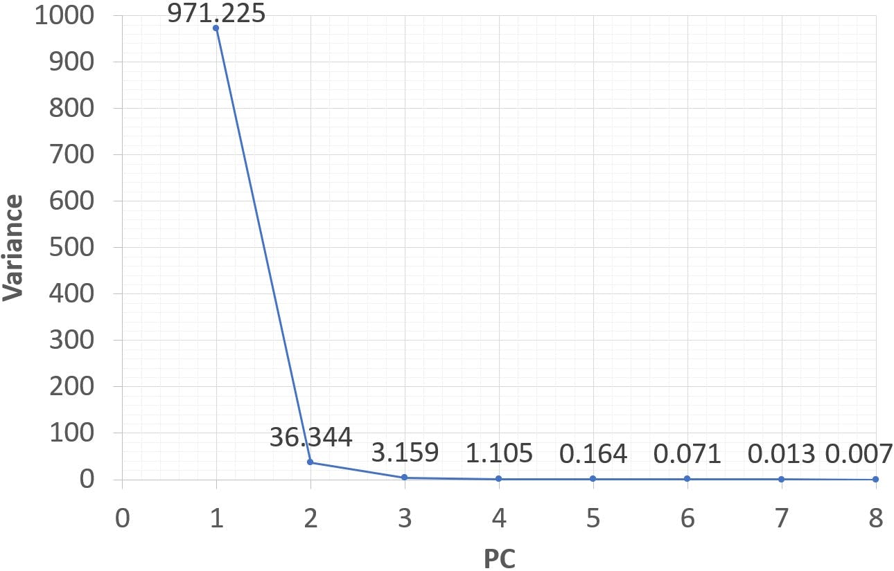
Figure 1: Scree plot of the 8 eigenvalues.
A scree plot displays the eigenvalues from highest to lowest value (therefore, in decreasing order of variance). Very often scree plots – like the one on Figure 1 – have an “elbow” beyond which variance levels off. The principal components “above” the elbow are generally retained, as they account for the greatest amount of variability. In the example above, only PC1 would be retained.
Loadings of the Principal Components
Each eigenvalue has an associated eigenvector, which forms the basis of a principal component. The resulting principal components are unique linear combinations of the eight original variables, and the coefficients of the variables in the linear combinations are called the “loadings” of the PCs. These are shown on Table 7.
Table 7: Loadings of eight selected variables on PC1 to PC8.
| Variable | PC1 | PC2 | PC3 | PC4 | PC5 | PC6 | PC7 | PC8 |
| MW | 0.990 | 0.043 | -0.050 | 0.089 | 0.019 | 0.072 | 0.019 | 0.036 |
| pKa | -0.001 | 0.020 | -0.021 | -0.079 | -0.034 | -0.160 | 0.983 | -0.010 |
| pKb | -0.004 | 0.012 | -0.025 | -0.173 | 0.977 | -0.065 | 0.010 | 0.107 |
| pKx | -0.055 | 0.992 | -0.068 | 0.089 | 0.001 | 0.010 | -0.012 | 0.009 |
| pl | 0.012 | 0.052 | 0.954 | 0.134 | 0.055 | 0.237 | 0.071 | 0.064 |
| logD | 0.013 | 0.057 | -0.057 | -0.758 | -0.114 | 0.615 | 0.035 | 0.163 |
| Polar | 0.111 | 0.077 | 0.261 | -0.547 | -0.157 | -0.728 | -0.162 | 0.185 |
| NV | 0.061 | 0.040 | 0.099 | -0.239 | 0.064 | -0.022 | -0.029 | -0.960 |
PC1 has a very strong loading from MW, and much weaker contributions from Polarity, normalised Volume, and pKx, the pK of the amino acid side chain. pKx is the major contributor to PC2, which has much lower coefficients for logD, pI and Normalised Value. pI is the major contributor to PC3, which also has a significant coefficient for Polarity.
These contributions are often visualised on “loading plots”, such as Figure 2 for PC1 and PC2, which simplify the interpretation of the principal components being plotted in terms of the original variables:
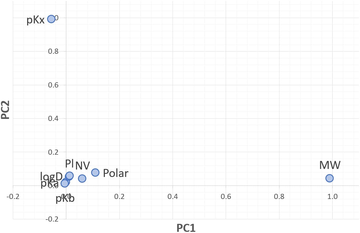
Figure 2: Loading plot for PC1 versus PC2.
In this graph, the horizontal axis indicates the contribution of each variable to PC1, and the vertical axis represents the contribution to PC2. Those variables close to zero (lower left corner of the plot) have small loadings on both principal components. MW has a strong loading on PC1 (close to one), but very weak on PC2 (close to zero). The opposite is true for pKx and PC2.
In a very real sense, PC1 is equal to MW, “complemented” with Polarisability and Nominal Volume. If we plot the amino acids along PC1 (the “scores” of the amino acids on PC1, which we will plot in the next section) we should see small, light, non-polar amino acids on the lower values; whereas bulkier and more polarisable amino acids should have higher PC1 scores.
PC2 can be described as pKx “decorated” with pI and Polarisability. This axis should allow us to differentiate between neutral and polar or ionisable amino acids, as it encodes information related to the chemical properties of the side chains. PC3 should further enhance this classification and allow us to separate neutral, acidic, and basic amino acids.
Scores
After computing the loadings of the original variables on the principal components, the twenty amino acids can be “mapped” onto the new system of coordinates, by applying the linear combinations that define each PC to the values of each amino acid. The new coordinates are called “scores”.
For example, PC1 is defined as:

The score of Alanine on PC1 is therefore:

The complete table of scores is shown below:
| Name | PC1 | PC2 | PC3 | PC4 | PC5 | PC6 | PC7 | PC8 |
| Alanine | 88.12 | 24.66 | 2.13 | 5.88 | 10.49 | -0.92 | 2.74 | 4.96 |
| Arginine | 174.23 | 21.99 | 6.01 | 7.34 | 10.55 | -0.89 | 2.53 | 5.01 |
| Asparagine | 131.19 | 26.70 | 0.61 | 8.60 | 10.18 | -1.22 | 2.53 | 4.90 |
| Aspartic acid | 132.99 | 10.40 | -1.03 | 6.42 | 10.78 | -1.20 | 2.53 | 4.93 |
| Cysteine | 120.93 | 14.52 | 1.40 | 5.79 | 9.35 | -1.00 | 2.46 | 5.01 |
| Glutamic acid | 147.14 | 11.84 | -0.72 | 6.18 | 10.84 | -1.49 | 2.68 | 4.94 |
| Glutamine | 145.37 | 27.54 | 0.75 | 8.22 | 10.49 | -1.54 | 2.61 | 4.93 |
| Glycine | 73.95 | 23.84 | 2.25 | 6.30 | 10.60 | -0.93 | 2.79 | 4.98 |
| Histidine | 155.26 | 14.28 | 3.42 | 6.78 | 10.59 | -0.88 | 2.57 | 4.89 |
| Isoleucine | 130.63 | 27.10 | 1.80 | 4.72 | 10.41 | -1.36 | 2.57 | 4.90 |
| Leucine | 130.64 | 27.10 | 1.78 | 4.75 | 10.33 | -1.45 | 2.55 | 4.88 |
| Lysine | 146.28 | 18.60 | 5.89 | 5.97 | 10.38 | -1.76 | 2.66 | 4.85 |
| Methionine | 148.64 | 27.93 | 1.06 | 6.09 | 10.19 | -1.43 | 2.56 | 5.20 |
| Phenylalanine | 164.75 | 28.84 | 0.54 | 5.46 | 10.17 | -0.95 | 2.44 | 4.83 |
| Proline | 114.34 | 26.11 | 2.05 | 5.84 | 11.55 | -1.03 | 2.34 | 4.98 |
| Serine | 104.08 | 25.36 | 1.42 | 7.47 | 10.32 | -1.16 | 2.65 | 4.90 |
| Threonine | 118.22 | 26.14 | 1.19 | 7.33 | 10.25 | -1.03 | 2.54 | 4.80 |
| Tryptophan | 203.99 | 30.94 | 0.24 | 6.12 | 10.67 | -1.01 | 2.76 | 4.95 |
| Tyrosine | 181.29 | 19.77 | 0.93 | 5.57 | 10.31 | -0.80 | 2.73 | 4.90 |
| Valine | 116.45 | 26.27 | 1.83 | 5.17 | 10.39 | -1.14 | 2.60 | 4.89 |
As expected, the scores on PC1 for the amino acids are not very different from their molecular weights. The small differences are the combined effects of the other variables on the calculation of PC1. However, we cannot give PC1 units of “g/mol”, since it is a combination of eight distinct physical magnitudes.
The scree plot and eigenvalues table suggested that PC1 would suffice to describe 96% of the information contained in the original data set. The graphical representation of the twenty amino acids on PC1 is displayed on the following figure:
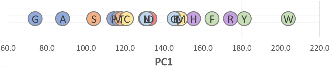
Figure 3: PC1 scores of twenty amino acids.
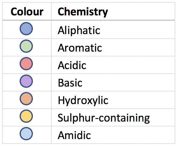
We predicted that small, neutral amino acids would be placed on the lower end of PC1, and increasingly bulkier and more polarisable species would appear at higher PC1 values. Whilst this is correct, PC1 alone is not able to separate the different chemical categories of amino acids, represented by the coloured icons:
The reason is clear: Molecular Weight values are so much bigger than the rest of variables, that they dominate the computation of the first principal components. Although MW accounts for a very large amount of variance, it does not encode the chemical information reflected in the other variables. This subtle information, which could arguably be of high value in many situations, is “displaced” to the lower rank principal components (PC2, PC3, etc.)
When deciding which principal components should be retained and which discarded, the scree plot rule is somewhat simplistic. It should always be supplemented with a brief exploration of loadings and scores to better understand how the information is being represented in the new PC space.
Standardised Variables and the Correlation Matrix
Most statistical packages offer the option to standardise the original variables as the first step prior to PCA. Standardisation, or normalisation, consists in calculating the mean and standard deviation of each variable, and use the to transform the data points:
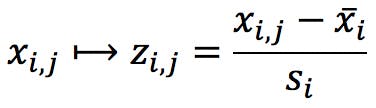
Where ![]() and
and ![]() are the mean and standard deviation of variable i, and xi,j is the value of variable i for object j. For example, the variable MW would be standardised as follows:
are the mean and standard deviation of variable i, and xi,j is the value of variable i for object j. For example, the variable MW would be standardised as follows:
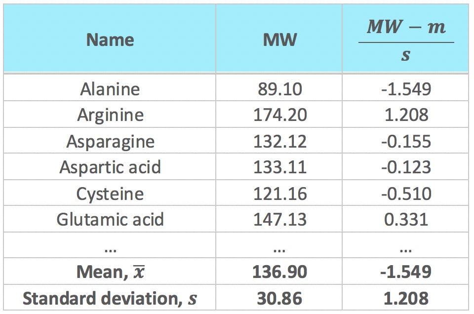
Standardisation is generally used when there are big differences in absolute values and (or) ranges between the variables. Our data set is a good example: MW values are one order of magnitude greater than those of NV; and they range between 75.07 g/mol and 204.23 g/mol, whereas the range of NV is much smaller, 0 – 8.08 units. Consequently, as we have seen in previous sections, MW will naturally have much more weight on the calculation of the first few PCs than NV – which may or may not be a desirable effect. By subtracting the mean and dividing by the standard deviation, these large differences are negated: all standardised variables will have an average of zero, and a variance of 1, which ensures they have equal weight on the calculation of PCs.
After standardising the data, the covariance matrix becomes a correlation matrix: diagonal elements are 1 and element above and below the diagonal indicate the pairwise correlation between the variables:
Table 9: Correlation matrix for eight selected variables (standardised).
| MW | pKa | pKb | pKx | pI | logD | Polar | NV | |
| MW | 1.000 | -0.119 | -0.298 | -0.268 | 0.204 | 0.425 | 0.968 | 0.979 |
| pKa | -0.119 | 1.000 | 0.268 | 0.621 | -0.141 | 0.500 | 0.015 | -0.007 |
| pKb | -0.298 | 0.268 | 1.000 | 0.228 | -0.147 | 0.209 | -0.232 | -0.221 |
| pKx | -0.268 | 0.621 | 0.228 | 1.000 | 0.095 | 0.211 | -0.147 | -0.154 |
| pI | 0.204 | -0.141 | -0.147 | 0.095 | 1.000 | -0.008 | 0.331 | 0.299 |
| logD | 0.425 | 0.500 | 0.209 | 0.211 | -0.008 | 1.000 | 0.565 | 0.552 |
| Polar | 0.968 | 0.015 | -0.232 | -0.147 | 0.331 | 0.565 | 1.000 | 0.996 |
| NV | 0.979 | -0.007 | -0.221 | -0.154 | 0.299 | 0.552 | 0.996 | 1.000 |
Scree Plot
The eigenvalue table and scree plot show a remarkable departure from the previous analysis:
| Eigenvalue | λ | % Variance | % Additive |
| 1 | 3.469 | 43.36% | 43.36% |
| 2 | 2.089 | 26.11% | 69.47% |
| 3 | 1.057 | 13.22% | 82.68% |
| 4 | 0.782 | 9.77% | 92.46% |
| 5 | 0.351 | 4.39% | 96.84% |
| 6 | 0.247 | 3.08% | 99.93% |
| 7 | 0.004 | 0.05% | 99.98% |
| 8 | 0.001 | 0.02% | 100.00% |
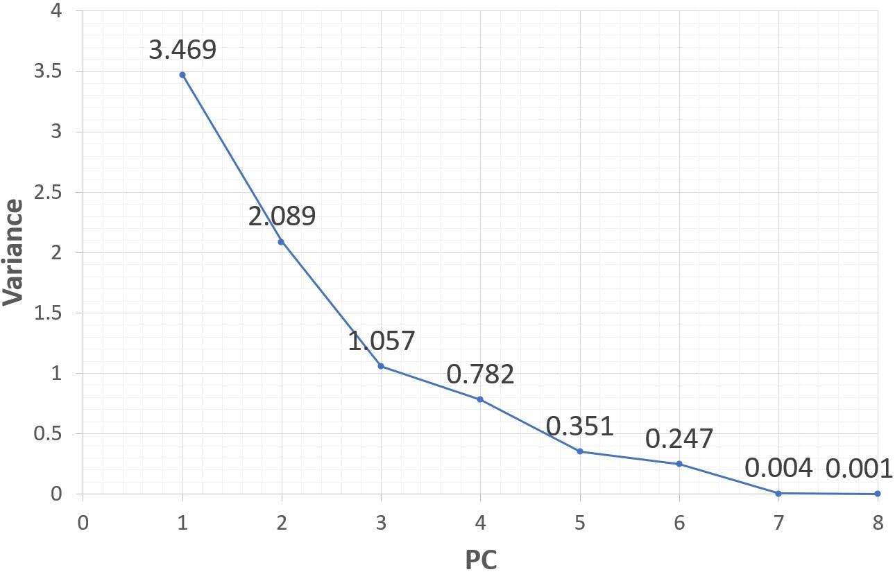
Figure 4: Scree plot of eight principal components (standardised variables)
Calculated on standardised variables, the first principal component only contains 43% of the variance. 26% is ascribed to PC2, 13% to PC3, etc. it is clear that we will need to retain a larger number of PCs to represent the system. However, the scree plot does not have the sharp “elbow” we saw in the previous calculation. How is a decision made in these cases? Although a deeper analysis of loadings and scores is always a sound idea, it is common in practice to apply a “Pareto” criterion, and retain those principal components that accumulate 80% or more of the variance. In this example, PC1, PC2 and PC3 could be considered satisfactory.
Loadings
The loadings chart for PC1 and PC2, and the loadings table for the first three principal components are shown below:
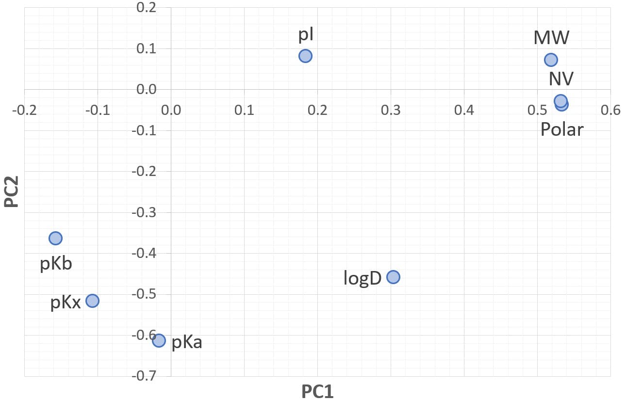
Figure 5: Loading chart for PC1 and PC2
Table 10: Loadings for PC1, PC2, PC3 (standardised variables)
| Variable | PC1 | PC2 | PC3 |
| MW | 0.519 | 0.072 | 0.111 |
| pKa | -0.016 | -0.614 | -0.030 |
| pKb | -0.157 | -0.364 | 0.254 |
| pKx | -0.107 | -0.517 | -0.455 |
| pI | 0.184 | 0.081 | -0.816 |
| logD | 0.304 | -0.458 | 0.222 |
| Polar | 0.534 | -0.037 | 0.000 |
| NV | 0.532 | -0.029 | 0.029 |
PC1 is almost equally shared between MW, Polarisability, and Normalised Volume: the factors that were secondary in our original analysis have now become much more prominent. PC2 is composed of pKa, followed closely by pKx and logD. pKb has a smaller, but significant, contribution. PC3 is still strongly dominated by pI, but it also receives a strong contribution from pKx.
It should be noted that these variables have negative loadings: as the variables increase in value, PC2 and PC3 would decrease. It is the magnitude of the loading, regardless of its sign, that determines which variables are most strongly associated with each PC.
These combinations the variables seem almost natural. It is often said that PCA reveals the hidden structure of a data set, and can uncover latent variables that may have not been initially obvious. For example, it seems appropriate to assimilate PC1 to the “bulk”; PC2 to the “polarity”; and PC3 to the “acid-base character” of the amino acids. We might even prefer these more descriptive names, instead of PC1, PC2 and PC3.
Scores
Table 11: Scores of twenty amino acids on PC1, PC2, PC3 (standardised variables)
| Name | PC1 | PC2 | PC3 |
| Alanine | -2.559 | -1.201 | -0.385 |
| Arginine | 2.518 | 2.021 | -2.018 |
| Asparagine | -0.983 | 1.203 | -0.691 |
| Aspartic acid | -1.082 | 1.904 | 2.357 |
| Cysteine | -0.570 | 2.128 | 0.398 |
| Glutamic acid | -0.186 | 0.990 | 2.235 |
| Glutamine | -0.175 | 0.339 | -0.514 |
| Glycine | -3.556 | -1.039 | -0.518 |
| Histidine | 1.007 | 2.347 | -0.107 |
| Isoleucine | 0.255 | -1.885 | 0.096 |
| Leucine | 0.262 | -1.788 | 0.053 |
| Lysine | 1.187 | 0.904 | -1.489 |
| Methionine | 0.791 | -0.934 | -0.102 |
| Phenylalanine | 2.014 | -1.009 | 0.327 |
| Proline | -1.375 | -0.806 | 0.238 |
| Serine | -2.163 | 0.146 | -0.646 |
| Threonine | -1.246 | 0.358 | -0.521 |
| Tryptophan | 3.833 | -2.087 | 0.435 |
| Tyrosine | 2.708 | -0.089 | 0.923 |
| Valine | -0.680 | -1.502 | -0.070 |
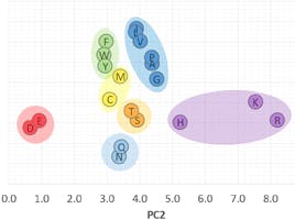
This table of scores allows us to visualise the twenty amino acids in a three-dimensional space, as seen in the figure below (created with Plotly Chart Studio) where each amino acid has been labelled according to the colour scheme seen earlier:
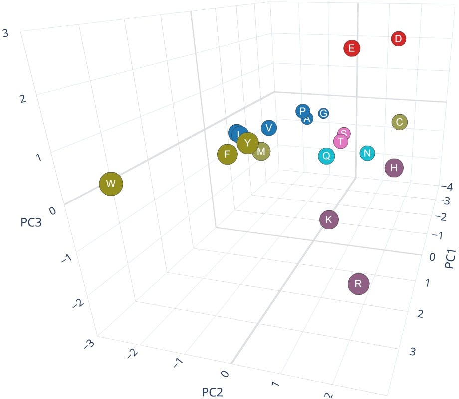
Figure 6: 3D scatter plot of PC1, PC2, PC3
The chart clearly shows that the combination of the three principal components is not only able to sort the objects in increasing molecular weight (along the PC1 axis), but it also reveals distinct groups and trends, that correspond to the seven categories of amino acids.
Displaying the scores on two-dimensional scatter plots clearly shows the ability of PCA to show patterns in the data set and to simplify further analysis:
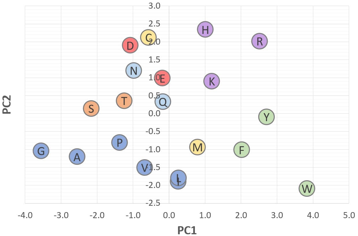
Figure 7: 2D scatter plot of "Polarity" (PC2) v "Bulk" (PC1)
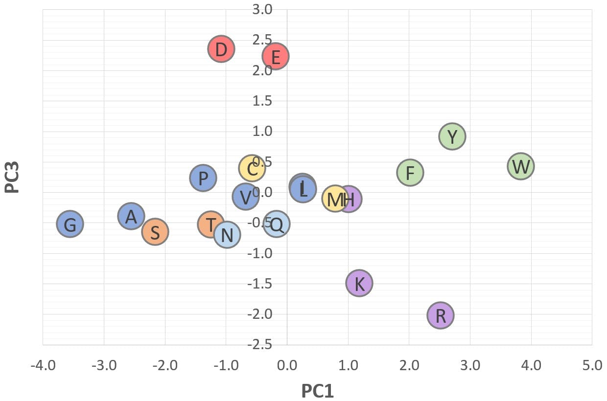
Figure 8: 2D scatter plot of "Acid-Base" (PC3) v "Bulk" (PC1)
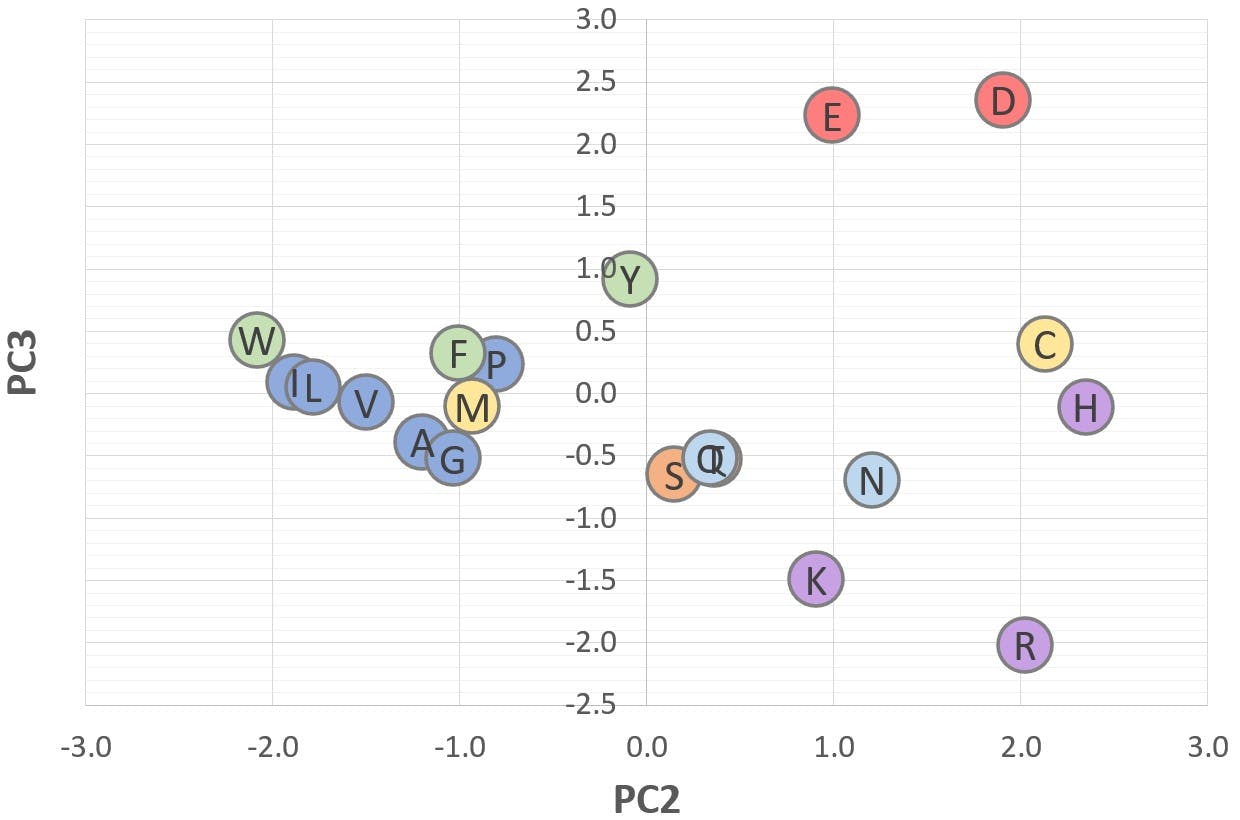
Figure 9: 2D scatter plot of "Acid-Base" (PC3) v "Polarity" (PC2)
These graphs illustrate a potential application of PCA: Figure 6 shows that amino acids with a positive PC2 are polar or ionisable in nature, whereas amino acids with a negative PC2 are aliphatic or aromatic. Figure 7 shows that acidic amino acids have a positive PC3, whereas basic amino acids have a negative PC3. Those with a PC3 close to zero are non-ionisable.
Working with raw or standardised variables are not the only possibilities: one could apply judicious transformations to the data if they are deemed to be of benefit. For example, Snyder et al. developed in the early 2000s a method for HPLC column characterisation, widely known as the “Hydrophobic Subtraction Model” (J. Chrom. A, 961, 2002, 171-193). The aim of the model was to quantify the different retention mechanisms involved in a chromatographic separation: hydrophobic interaction, ion exchange, shape selectivity, etc. They realised early on that hydrophobic interaction had an overwhelming effect on the results, and they decided to “subtract” it by dividing all the other factors by the hydrophobic contribution. Dividing pKa, pKb, pI… by the molecular weight of the amino acid may not be appropriate in our data set (I am not sure “pI per mass unit” makes any physical sense) but other strategies could well be interesting.
Outliers
Outliers are observations that lie outside of the general pattern of a distribution or mathematical model. In linear regression, for example, outliers can be detected by calculating “standardised residuals”:
Where the residual, ri, is defined as the distance between the experimental point yi and the regressed value, ![]() . After computing all the residuals, the average
. After computing all the residuals, the average ![]() and standard deviation sr can be calculated, and the residuals can be standardised thus:
and standard deviation sr can be calculated, and the residuals can be standardised thus:
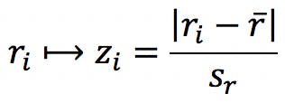
Any points with standardised residuals beyond a critical value are potential residuals and should be investigated further.
The multivariate equivalent to standardised residuals is the Mahalanobis Distance (MD), named after its creator, Prasandra Mahalanobis:
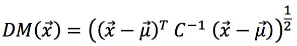
Here, ![]() is the object under investigation (e.g. each one of our amino acids) in the principal component space.
is the object under investigation (e.g. each one of our amino acids) in the principal component space. ![]() is therefore the vector of eight scores for a particular amino acid. For example, the vector “alanine” is:
is therefore the vector of eight scores for a particular amino acid. For example, the vector “alanine” is:

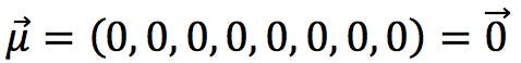
![]() represents the centroid of the objects in PC space: a vector whose coefficients are the average of each PC. For standardised data, the calculation is simplified because the average of each PCs is zero:
represents the centroid of the objects in PC space: a vector whose coefficients are the average of each PC. For standardised data, the calculation is simplified because the average of each PCs is zero:
Finally, C -1 is the inverse of the Covariance matrix. For standardised data, this is the inverse of the Correlation matrix:
| 286.938 | 7.249 | 8.660 | 9.306 | 37.263 | 44.122 | -9.106 | -303.938 |
| 7.249 | 2.826 | 0.050 | -1.194 | 1.646 | 0.220 | -7.588 | -0.307 |
| 8.660 | 0.050 | 1.630 | 0.329 | 0.921 | 0.637 | 4.154 | -12.830 |
| 9.306 | -1.194 | 0.329 | 2.354 | 0.437 | 1.257 | 5.404 | -14.889 |
| 37.263 | 1.646 | 0.921 | 0.437 | 6.595 | 6.286 | -10.671 | -31.013 |
| 44.122 | 0.220 | 0.637 | 1.257 | 6.286 | 9.537 | -7.009 | -43.025 |
| -9.106 | -7.588 | 4.154 | 5.404 | -10.671 | -7.009 | 189.262 | -170.797 |
| -303.938 | -0.307 | -12.830 | -14.889 | -31.013 | -43.025 | -170.797 | 496.522 |
The Mahalanobis distances for all twenty amino acids are:
| Name | MD | MD critical | p Value |
| Alanine | 2.299 | 15.507 | 0.970 |
| Arginine | 3.277 | 15.507 | 0.916 |
| Asparagine | 2.543 | 15.507 | 0.960 |
| Aspartic acid | 2.787 | 15.507 | 0.947 |
| Cysteine | 3.514 | 15.507 | 0.898 |
| Glutamic acid | 2.903 | 15.507 | 0.940 |
| Glutamine | 2.531 | 15.507 | 0.960 |
| Glycine | 2.922 | 15.507 | 0.939 |
| Histidine | 2.269 | 15.507 | 0.972 |
| Isoleucine | 1.885 | 15.507 | 0.984 |
| Leucine | 2.100 | 15.507 | 0.978 |
| Lysine | 3.591 | 15.507 | 0.892 |
| Methionine | 3.527 | 15.507 | 0.897 |
| Phenylalanine | 2.673 | 15.507 | 0.953 |
| Proline | 3.722 | 15.507 | 0.881 |
| Serine | 1.719 | 15.507 | 0.988 |
| Threonine | 2.202 | 15.507 | 0.974 |
| Tryptophan | 3.180 | 15.507 | 0.923 |
| Tyrosine | 2.550 | 15.507 | 0.959 |
| Valine | 1.470 | 15.507 | 0.993 |
The critical Mahalanobis distances and p values are given by the Chi-squared distribution. In Excel, these are calculated as:
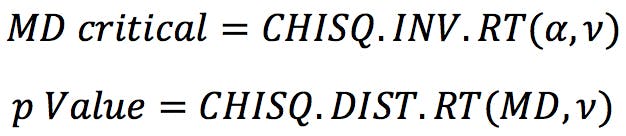
Where α is significance (set to 0.05 in this example) and v is degrees of freedom, which is equal to the number of PCs, 8. Our calculations indicate that none of the amino acids is an outlier. In other words, they all fit well within the method.
Conclusions
After a detailed introduction to the algebra behind Principal Components Analysis, this instalment is focused on some of the practical aspects of the technique, such as dealing with missing data, or highly correlated – and therefore potentially redundant – variables.
Most statistical packages enable the user to apply basic transformations to the data set prior to PCA. One of the most common options is to standardise the variables, which is commonly carried out when there are large disparities in absolute values and variances. We have demonstrated how this technique modifies the resulting principal components, and given general guidelines on how to use it.
Finally, the most important aspect of PCA is to interpret the results. We have discussed at length some graphical and statistical tools, including Mahalanobis distances to evaluate the presence of outlier objects.
As ever, I hope this article has been enlightening and useful. Questions and comments are welcome, and please do not hesitate to contact us for further information.
Related articles