03 Oct 2017
Solvent Choice for GC Injection
I guess we all have our ‘go to’ solvents for our work in GC, and most of the time this will be based on the availability of the solvent and the chemical nature of our samples. Polar samples (analytes) generally need a more polar solvent (methanol for example) and less polar analytes a less polar solvent (n-hexane or heptane for example). Sometimes we might even use an intermediate polarity solvent when we aren’t sure of the analyte composition, ethyl acetate is a popular choice in this instance.
I talk to many folks involved in GC and the conversations around sample preparation and the choice of ultimate sample diluent are almost always around the chemistry of the sample (matrix) or the analyte and the requirements to properly solubilise the sample.
But there are so many more issues to consider when choosing the appropriate sample solvent and setting some of our critical method variables. I’ve given a short treatment of these considerations in this instalment so you might be better informed when developing, optimising, transferring or troubleshooting your GC methods.
Sample Solvent (Diluent) and Injection Volume
The sample diluent has a direct effect on the amount of sample which can be injected into the GC under a given set of inlet conditions.
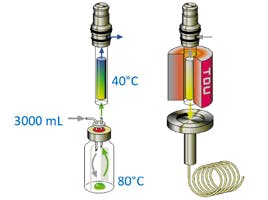
As the sample is rapidly introduced into the GC inlet via the autosampler syringe, there is a rapid (explosive) evaporation of the sample solvent which transfers the sample molecules into the gas phase. The degree of expansion will depend upon the nature of the sample solvent (i.e. its expansion co-efficient), and the inlet temperature and pressure, which is dictated by the combination of the liner size and the carrier gas flow rate through the inlet.
If the sample size (the number of microliters of sample you chose to inject) is too large, and other operating variables are not favourable, the gas phase sample will exceed the volume of the inside of the inlet liner, and the gas phase sample will contact the underside of the septum and ‘spill’ over into the carrier gas inlet and septum purge lines. As these lines are not heated (other than the portions directly inside or next to the inlet), then the gas phase sample will condense, leaving some of your analyte deposited within the pipework of your sample inlet system.
If one were to then inject a ‘blank’ solvent, under the same circumstances, the same overfilling phenomenon would occur, and just as a wave ‘laps’ the seaweed and other detritus from a beach, some of the previously deposited sample components within the pipework may be drawn back into the inlet and make their way into the column. We would be presented with a mini version of the previous chromatogram which we describe as ‘carry-over’ and which is a major cause of quantitative irreproducibility in capillary gas chromatography. Chromatographers call this phenomenon ‘backflash’ (Figure 1).
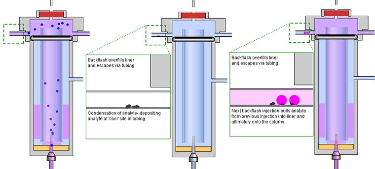
Figure 1: The principles of sample ‘backflash’. A – the solvent volume is too large to be contained in the inlet liner and ‘spills’ over into the inlet tubing. B – The analyte condenses in an unheated region of tubing. C – the next backflashed injection solvent vapour solubilises the deposited analyte and carries it back into the inlet and subsequently on to the column – resulting in carry-over.
So – how does one decide on the proper injection volume or the operating variables which will avoid this insidious carry-over effect?
Well we typically use software calculators to assess the correct amount of sample to inject and the appropriate inlet temperature and pressure. The calculator needs to know the nature of the solvent and its expansion co-efficient in order to calculate the volume of gas created under a given set of conditions, from a given volume of solvent injected into the system. It will also need the liner volume (easily calculated or requested from suppliers) and the temperature and pressure of the inlet, which of course you can get from the GC system.
Content on this page requires a newer version of Adobe Flash Player.

Figure 2: An example Backflash Calculator (taken from CHROMacademy.com). These simple software calculators are also available from most GC and GC column manufacturers.
These calculators are very useful as they allow one to assess the required changes to the operating conditions in order to avoid backflash, or on a more positive note, to assess how much sample can be injected without risking carry-over, if one wants to improve the sensitivity of a method.
Further, the calculator can be used to make informed choices on the detector temperature setting required for a particular method, alongside the general information that one might have about the boiling points of the higher boiling sample components.
The calculator can also be used to assess the effects of increasing the head pressure (carrier gas flow), during the moment of sample injection which constrains the expansion of the sample solvent plug, which is known as ‘pressure pulsed injection’, a strategy which is also used to increase the volume of sample injected without risking backflash and hence analyte carry-over.
Diluent effects on peak shape
During the initial phase of a splitless injection, the column is cool (40 – 70°C typically) and the sample solvent is allowed to condense on the stationary phase on the inner wall of the capillary column. Due to the reduced vapour pressure caused by the flowing carrier gas, the solvent evaporates and ‘concentrates’ the dissolved analytes into a sharp band.
This effect, known as solvent focussing, helps to overcome the very broad peak shapes associated with splitless injection into a hot oven, caused by the prolonged time taken to move the sample vapour from the inlet to the column under splitless conditions.
The peak focussing effects rely upon the solvent forming a contiguous (uninterrupted) film on the inner wall of the capillary column. If the polarity of the column stationary phase is not well matched with the polarity of the sample diluent, this film formation can fail and ‘pooling’ of solvent can occur which results in a non-contiguous film and very poor peak shape.
These effects along with the resulting chromatograms can be seen in Figure 3.
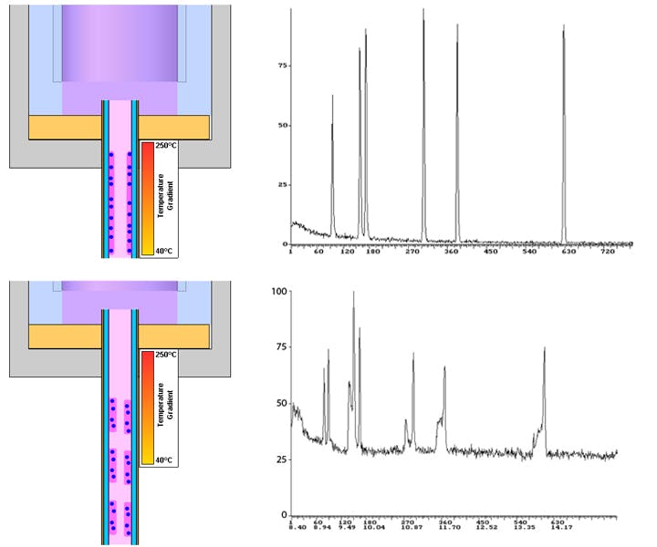
Figure 3: Splitless injection of a test compound mix under splitless conditions. Top – good peak shape obtained from matched stationary phase and sample diluent solvent polarity (5% phenyl polydimethylsiloxane phase with dichloromethane as sample solvent) Bottom – poor peak shape obtained from stationary phase, sample diluent solvent polarity mismatch (5% phenyl polydimethylsiloxane phase with methanol as sample solvent)
These effects can also occur to a lesser extent in split injection, however they are typically much less severe.
Typically one should avoid extremes such as using methanol as a sample diluent with non-polar GC stationary phases such 100% polydimethylsiloxane or n-hexane as a sample diluent when using polar phases such as waxes. However, minor effects can also be seen when using intermediate polarity phases or solvents and one should take care to match the solvent polarity with that of the stationary phase.
So, the next time your reach for the solvent bottles to dissolve or reconstitute your sample prior to loading it into the GC vial – just stop a moment and run through the considerations above. Make an informed solvent choice – your chromatography will be all the better for it!
Related articles