21 Sep 2017
System and Column Volumes in HPLC - we still haven’t got the message!
Some modern HPLC systems resemble spacecraft in terms of their technology, designed as they are to operate to the highest efficiencies, compared to traditional systems.
However, I still see countless examples where high efficiency columns are used on systems which are not matched and cannot support the highest efficiencies offered by the column.
There are many factors to consider when considering the optimum efficiency obtainable from a system / column combination and I’ve outlined below some of the variables which can be easily controlled within the laboratory and data acquisition variables which need to be considered.
For reference, I’m not going to consider Capillary or Nano columns here, as to take advantage of these technologies you will have already considered all of the information presented here.
You will need to know the extra column volume associated with your HPLC column which, as a first approximation, can be calculated in the following way;
| 2.1mm i.d. – column length (mm) x 2 = column void volume (Vm) (μL) |
| 50mm long 2.1 mm i.d. column has a void volume of approx. 100 μL |
| 3.0mm i.d. – column length (mm) x 5 = column void volume (Vm) (μL) |
| 100mm long 3.0 mm i.d. column has a void volume of approx. 500 μL |
| 4.6mm i.d. – column length (mm) x 10 = column void volume (Vm) (μL) |
| 150mm long 4.6 mm i.d. column has a void volume of approx. 1500 μL |
The fact of the matter here is that shorter, narrower columns and those packed with highly efficient packing materials (<2mm or superficially porous particles), need to be used with HPLC systems whose extra column volumes are low, to avoid the system being the dominant factor in determining the maximum achievable efficiency.
The extra column volume (ECV) within a system is additive alongside the dispersion that occurs within the column in determining the peak volume (peak width) and there is a very nice rule of thumb which states that the ECV of the system should be less than half of the total peak width in order to achieve more than 90% of the column resolving power.
This is what we should be aiming for.
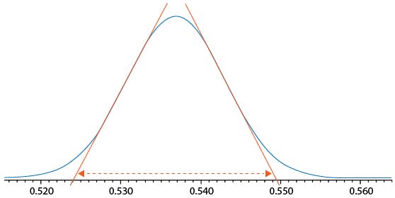
Figure 1: Measuring peak volume to assess system dispersion requirements.
In Figure 1 the chromatographic peak volume can be estimated by drawing tangents as shown to estimate 4σ peak width – in this case the peak width is 0.5495 – 0.5240 mins = 0.0255 mins and the flow rate was 600 μL per minute giving an estimated peak volume of 15.3 μL. This would dictate that the total system extra column volume (ECV) should be less than 8 μL (approx.) in order to achieve the optimum resolving power of the column / system combination.
Some typical maximum allowable ECV contributions for columns of various dimensions are shown in Table 1.
| Column Dimensions (L x i.d., mm) |
Maximum Extra Column Volume (μL) |
| 100 x 4.6 50 x 4.6 100 x 3.0 50 x 3.0 100 x 2.1 50 x 2.1 30 x 2.1 |
35 25 15 10 7 5 4 |
Table 1: Maximum allowable extra column volume for columns of various dimension.
So, what do we need to take care of in order to optimise our experiments from a practical perspective?
Well, I’ve compiled a brief list below of the items that we review on each system after measuring the ECV to reconcile the measured value against what is calculated;
- Volume of sample injected
- Tubing from autosampler to column heat exchanger
- Column heat exchanger
- Tubing from heat exchanger to column and column to detector
- Detector internal tubing volume (often negligible but sometimes not!) and flow cell volume
- Fittings and in-line filters / unions etc.
So – how can you estimate the ECV value;
- Known
- Use Table 2 to calculate
- Should be written on the heat exchanger or in your manufacturers literature
- See 2 above
- From manufacturer; cell volume will be written on the cell or via part number
- Zero contribution from fittings if zero dead volume type used
| Tubing internal diameter (mm) |
ECV contribution (μL/cm) |
| 0.127 0.178 0.229 0.254 |
0.13 0.25 0.41 0.51 |
Table 2: Volume contribution from tubing of various internal diameter.
To calculate the ACTUAL extra column volume of the system, replace the column with a zero dead volume union or capillary restrictor and inject an aliquot of 0.1% v/v acetone in water and monitor at 270nm with your UV detector. Measure the 4s peak width and calculate the peak volume as per Figure 1 above. This value is the ECV value for the system you are using.
One should carefully consider, and reduce where possible, the tubing length and internal diameter being used, especially between the column and detector, the number of unions and any in-line filters or couplings which may not be necessary. Our earlier example with the 8 mL maximum ECV constraint would start to suffer problems if any more than 32cm of 0.178mm i.d. tubing is present in the whole system!
You should note above the comment regarding zero contribution from ZDV unions. Well this is only true if the connection is properly made! Ensure that the tubing is fully butted up inside the fitting and that it remains that way during the tightening operation – basic good practice that often is not followed. Also remember that PEEK fittings deform only so many times and old PEEK column nuts will eventually lose their ability to deform to the internal volume of the column end fitting.
Given the constraint of keeping below 8 mL ECV, one may also need to consider for our system above, the required injection volume. Clearly injection volumes need to be scaled when using lower volume columns and a nice estimate of maximum injection volume is around 15% of the peak volume. So restricting injection volume to no more than 2.25 mL would be sensible for our example here. If scaling down a method to a smaller column dimension, and assuming a constant particle porosity, then a simple scaling relationship is;
Vinj(2) = Vinj (1) x (i.d(1) x L(1) / i.d.(2) x L(2))
where Vinj (1) is original injection volume, i.d.(1) the internal dimeter of the original column and so forth…
Another very useful rule of thumb in reducing ECV and minimising peak dispersion to realise maximum efficiency is to restrict the flow cell of the detector to less than 10% of the calculated peak volume. In our previous example the peak volume was approx. 15 μL indicating a maximum flow cell volume of around 1.5 μL. This indicates the need for a flow cell based on light pipe principles which have very low internal volume whilst still maintaining good sensitivity.
Table 3 outlines the relative merits of flow cells of various dimensions;
| Cell Volume (µL) | Path Length (mm) | Signal to Noise ratio | Efficiency * |
| 13 5 2 0.08** |
10 6 3 6 |
++++ +++ ++ +++ |
+ ++ +++ ++++ |
* - ultimate efficiency depends upon the total system extra column volume and column dimensions
** - based on light pipe design
Table 3: Effect of flow cell volume on chromatographic performance.
The most surprising contributor to peak dispersion is the data acquisition parameters that we apply to a method. The data sampling rate can have a direct effect on peak width (efficiency) and as such these are important parameters which must be matched to the widths of peaks generated by various column dimensions.
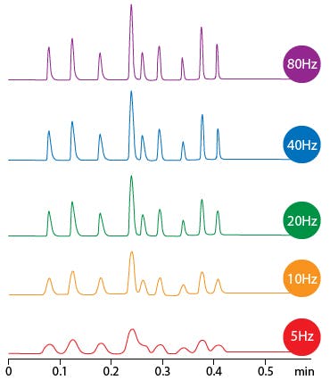
Figure 2: Effect of data sampling rate on peak shape and efficiency. Right – use of time constant to adjust noise, which is especially important in high frequency measurements.
However, data sampling rate is not the only important factor in determining peak width and variables such as bunch rate or time constant, i.e. the digital bunching and filtering applied by the detector, are also of importance and some guideline as to these variables are shown in Table 4.
| Column Dimensions (L x i.d., mm) |
Minimum Data Rate (Hz) | Maximum Time Constant (Sec.) |
| 50 x 4.6 50 x 3.0 50 x 2.1 |
10 20 20 |
0.16 0.16 <0.1 |
Table 4: Recommended data acquisition rates for columns of different internal diameter.
To conclude, Figure 3 shows the effect of extra column volume on a chromatographic separation using a column of 100 x 2.1mm with an ECV of 20 μL (bottom) and 80 μL (top).
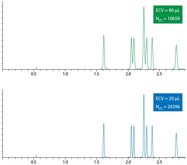
Figure 3: Effects on chromatographic performance of systems with varying extra column volume.
It should be clear from Figure 3 that the upper separation would not find favour in regular use and that the efficiency of peak 7 has fallen by more than half due to a 4x increase in system Extra Column Volume.
It is very important, when using reduced dimension HPLC columns and high efficiency particle morphologies, that the system volume and data acquisition parameters are optimised in order to realise the full efficiency benefits.
Related articles