04 Mar 2019
Core-Shell particles
In the late noughties we couldn’t avoid webinars, seminars, and online calculators extolling the virtues of the ‘new’ core-shell particle morphology. Used by HPLC column manufacturers, they promised higher performance at lower backpressures. Many of us wondered if this was a reaction to the introduction of sub 2μm HPLC particles and UHPLC instrumentation (around 2004), particularly the speed and efficiency which this approach brought to our industry.
Now, it would appear the hype around core-shell particles has died down. In fact, I’ve lately had trouble finding an online method translator — most manufacturers have core-shell versions of their popular phases from their fully porous particle ranges. So, are we in danger of forgetting the advantages which core-shell particles can bring to methods which still use fully porous particles? Or, put differently, why do 5μm or 3μm fully porous particles still exist? And why hasn’t everyone migrated their methods to this superior technology? After all, with 2.7μm (or similar) and 5μm core-shell particles widely available why wouldn’t we all want to update our legacy methods, or seek to develop new methods using core-shell particles?
I really can’t answer this question, although I suspect that there are many legacy methods which work perfectly well on fully porous particles; therefore, there is no real driver to change. That being said, I see so many scientists struggling with methods where an improvement in efficiency (and, resultantly, resolution) would deliver significant benefits — solving issues with their troublesome methods or identifying how shortened analytical run times may help with throughput problems. These are the people I have in mind with this piece — those who seek to improve or replace existing methods on a limited budget for new instruments.
As well as a refresher on the simple maths required to undertake method transfer from fully porous particles (FPP) to superficially porous particles (SPP) I’m going to impose a further constraint by working within the new USP General Chapter proposition <621> which is currently in draught form [1]. For a more detailed explanation of the proposed changes to Chapter <621> see reference [2].
To translate the various method parameters from the FPP to the SPP column, one might use the following equations;
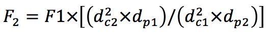
Flow Rate
(Equation 1)
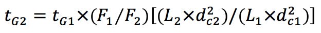
Gradient Segment Times
(Equation 2)
When changing column or particle size dimensions, for USP methods we need to comply with the requirements that;
L/dp = -25% to +50%
or
N = -25% to +50%
That is, the column length (L) to particle size (dp) ratio must not fall outside these limits.
In this case we wish to translate the USP method for Lanzoprazole and it impurities, which uses a 150 x 4.6mm column with 5μm FPP, to an SPP column which uses 2.7μm particles.
Typically, we can choose columns of 100, 75, or 50mm in length. We need to decide which of these columns would comply with the requirements of Chapter <621>
| L | dp | L/dp ratio | % change |
| 150 | 4.6 | 32,600 | - |
| 100 | 2.7 | 37,100 | +14 |
| 75 | 2.7 | 27,800 | -15 |
| 50 | 2.7 | 18,500 | -44 |
So, we can see that the 100 or 75mm columns are available as options when switching to 2.7μm SPP formats. Let’s assume that we wish to take full advantage of the speed gains offered by SPP particles and that we will opt for the 75mm column.
We can also reduce the internal diameter of the HPLC column, providing that the linear velocity of the eluent is maintained. To ensure that this is the case, we use Equation 2 to calculate the eluent flow rate.
Typically, we will be able to choose from 3mm or 2.1mm internal diameter columns; however, we must be careful when reducing internal diameter, as making large changes to the instrument dwell volume (VD) to column volume (VM) ratio has been shown to induce changes in selectivity when using gradient methods [3]. Whilst a detailed treatment of this topic is outside the scope of this discussion, I would urge you to seek further information from Reference 3, which also details which changes to the gradient program might be made in order to avoid selectivity issues when large changes in VD/VM are required.
We can estimate the interstitial volumes of both the SPP and FPPs if we know some facts about the materials in use. We might measure this directly by measuring the dead time (volume) of the system with and without the column installed.
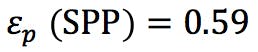
We also need to know the porosity ep of the particles (ask your manufacturer for this information) or we might estimate the porosity of the corresponding SPP using the relationship;
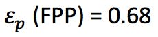 (information obtained from the manufacturer or estimated from dead time marker)
(Equation 3)
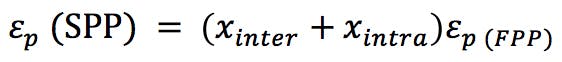
(Equation 4)
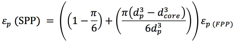
(SPP particle diameter = 2.7μm and core diameter = 1.7μm)
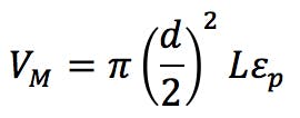
stimating the extra column volume for our three columns can then be achieved using;
(Equation 5)
If we assume the system dwell volume is around 300mL the VD/VM ratio changes here would be;
150 x 4.6 mm column using FPP VM = 1700μL, VD/VM = 0.18
75 x 3.0 mm column using SPP VM = 313μL, VD/VM = 0.96
75 x 2.1 mm column using SPP VM = 153μL, VD/VM = 1.96
We can estimate the required gradient adjustment required for the two reduced dimension columns using the following equation;
(Equation 6)
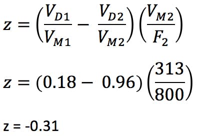
If the value for Z is negative, then the gradient needs to be started Z minutes prior to sample injection (possible with newer HPLC systems). If positive, an isocratic hold of Z minutes needs to be inserted at the start of the gradient.
Working through the various calculations, we arrive at the following sets of conditions;
Original Method;
Column – 150 x 4.6 mm 5μm (FPP)
Flow rate – 1 mL/min
Gradient –
| Time (mins) | Solution A (%) | Solution B (%) |
| 0 | 90 | 10 |
| 40 | 20 | 80 |
| 50 | 20 | 80 |
| 51 | 90 | 10 |
| 60 | 90 | 90 |
(A is 100% water, B is acetontrile:water:triethylamine (160:40:1) adjusted to pH 7.0 with phosphoric acid)
Translated method 1;
Column – 75 x 3.0 mm 2.7μm (SPP)
Flow rate – 0.79 mL/min (rounded to 0.8 mL/min) - Calculated from Equation 1
Gradient –
|
Calculated using Equation 6 Subsequent lines calculated using Equation 2 Equilibration time calculated using (10x column volume) / flow rate) |
Note that the gradient here needs to be started 0.3 minutes prior to sample injection to retain the selectivity. If this is not possible using your equipment, consider using the same internal diameter column as the original, but with reduced column length (i.e. 75 x 4.6mm in this case). Furthermore, the re-equilibration time has been calculated using 10x column volume which may be shortened but this needs to be assessed empirically.
Translated method 2;
Column – 75 x 2.1 mm 2.7μm (SPP)
Flow rate – 0.39 mL/min (rounded to 0.4 mL/min) - Calculated from Equation 1
Gradient –
|
Calculated using Equation 6 Subsequent lines calculated using Equation 2 Equilibration time calculated using (10x column volume) / flow rate) |
Here the gradient needs to be started 0.7 minutes prior to sample injection.
The chromtaograms obtained using these three methods are shown in Figure 1;

Figure 1: Resulting chromatogram with figures of merit for the original USP method for Lansoprazole impurities and the same method employed using Chapter <621> allowable changes and 2.7μm Superficially Porous Particles with 75mm x 3.0mm (middle) and 75 x 2.1mm (bottom)
Another important adjustment is the volume of sample injected. As column dimensions are reduced, and the particle morphology is changed, the amount of stationary phase available is reduced. This risks overloading the column, fronting peaks, plus reduced accuracy and reproducibility of quantitation. We have found the following formula very useful, which is based on a well-established mathematical relationship. However, it further reduces the injected volume by 30% to account for the marginally lower loadability of the superficially porous particles. Reducing by a further 30% is generally more than is required to account for the reduction in available surface area, and the injection volume may be increased empirically if extra sensitivity is required.
(Equation 7)
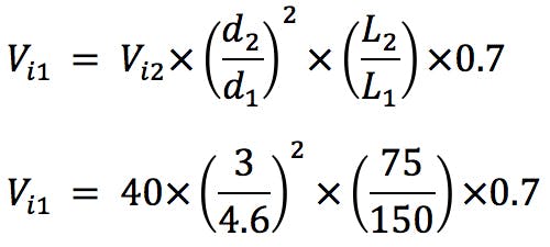
 (5μL used in practice for the 3mm i.d. column and 3μL used for the 2.1mm i.d. column)
Note that this formula is not recognised by USP <621> the current version of which (USP 40 – NF 35) says: ‘The injection volume can be adjusted as far as it is consistent with accepted precision, linearity, and detection limits. Note that excessive injection volume can lead to unacceptable band broadening, causing a reduction in N and resolution, which applies to both gradient and isocratic separations’. Therefore, the suitability of the injection volume using the method in Equation 7 should be assessed empirically.
From the chromatograms in Figure 1 it should be obvious that either of the superficially porous core-shell column methods are more than three times faster than the USP method using the original conditions. This improvement in speed is due to the increased efficiency of core-shell columns, which allow appreciably smaller columns to be used without compromising the efficiency and resolution of the separation. This increase in speed of analysis can be very important in high throughput laboratories.
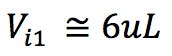
However, there are also situations in which the inherent efficiency increase achieved when using core-shell particles can be a great advantage. In the following example we used a system with a dwell volume of 300μL and extra column volume of 60μL, initially following the USP method. Figure 2 (top) shows that the resolution between the Lansoprazole and Lansoprazole RS A peaks would be unacceptable in a practical situation. Using the principles above, a method translation was produced which used a 2.7μm superficially porous particle with the same 150 x 4.6mm column dimension, which produced a significant improvement in resolution from 1.78 to 2.38, which may be usable in practice.
Figure 2: Resulting chromatogram with figures of merit, using a standard HPLC system, for the original USP method for Lansoprazole impurities (top) and the same method employed using Chapter <621> allowable changes and 2.7μm Superficially Porous Particles with the same column dimensions (bottom).
Using simple translation methods, we have demonstrated that chromatographic run times and quality of chromatography can be significantly improved by using superficially porous silica particles. Perhaps we should then ask our original question again — ‘why would a fully porous particle be used when the use of superficially porous particles brings so many benefits’? Surely it couldn’t be that the method translation effort is too much to bear?
Finally, perhaps we need to briefly consider the question of selectivity equivalence between the fully porous and superficially porous variants of manufacturers stationary phases. We have seen some variation in selectivity between FPP and SPP variants of nominally the same bonded phase from the same manufacturer. Whilst adjustments to the gradient profile to account for VD/VM ratio differences can help to address these issues, the fact remains that selectivity differences have been noted. Could this be a factor which makes the preferential use of SPPs a step too far for method translation? Of course, this would not be a problem if the SPP was used during the method development phase and we should also note the fidelity of selectivity between FPP and SPP variants are very good for some manufacturers.
References:
[1] C188676 (43(5) Harmonization Stage 4 General Chapter 621)
[3] http://www.chromatographyonline.com/translations-between-differing-liquid-chromatography-formats
Related articles