03 Oct 2017
Practical HPLC method development screening
Last time we discussed the various considerations for column selection when choosing HPLC columns for ‘Platform’ method development approaches.
I often get asked about the other important aspects of ‘screening’ in HPLC, which include the mobile phase composition, gradient parameters and flow rate – so that’s the theme of this instalment.
Mobile phase selection is key to getting a good insight into the selectivity which each stationary phase has to offer, and remember that this is a combination of the bonded phase ligand, the silica substrate and any post bonding treatments such as end-capping etc. Ideally we want to screen the sample with as wide a range of mobile phase chemistries as we can in order to fully map the selectivity possibilities, so this is typically going to involve changing modifier, pH and buffer type and strength.
The selectivity obtained using Methanol and Acetonitrile are often very different, especially where acidic, basic and/or aromatic analytes are involved, due to the different physico-chemical properties of these common HPLC solvents.
Most people will have seen the figure below but you may not have the accompanying data which highlights the major differences and how this might affect the various types of analyte that we deal with.
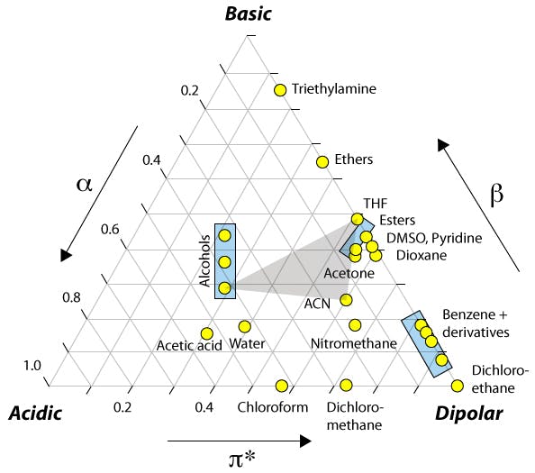
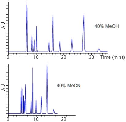
Figure 1: Selectivity (and retention) changes due to the differences in physico chemical properties of the organic modifier.
| Solvent | Dipole π* | Acidity α | Basicity β |
| MeOH | 0.28 | 0.43 | 0.29 |
| MeCN | 0.60 | 0.15 | 0.25 |
Table 1: Relative properties of Methanol and Acetonitrile which influence retention and selectivity in reversed phase HPLC.
The relative acidity and basicity of each modifier has different effects on the solubility of the analyte in the mobile phase relative to the stationary phase and hence selectivity between analytes. For this reason, a screen to investigate the selectivity ‘map’ for any separation should include chromatograms generated using both acetonitrile and methanol.
Next we need to consider pH and choice of buffer. Most of you will be aware that, for ionisable molecules, the pH of the eluent will affect the degree of analyte dissociation, and hence it’s retention, due to the relative decrease or increase in polarity as the molecule becomes more or less ionised. As all analytes have a different extent of dissociation at various pH values, then altering the mobile phase pH will alter the relative retention of each ionisable analyte and therefore the selectivity will alter.
Depending upon the nature of the analyte, one might want to choose acidic, neutral and basic pH to investigate a wide range of pH values, although if you are using modelling or optimisation software to assist your method development, the range of pH values used may need to be reduced in order to create a valid model.
This is the point at which many folks come unstuck, through poor selection of the buffer type and concentration. I’ve listed the pKa of some common buffers in Table 2. For maximum buffering capacity, one should get as close (with eluent pH) to the buffer pKa value as possible, but certainly we should try to remain within +/- 1 pH of the buffer pKa. If this rule is followed, then a buffer strength of 10mM may well be enough to effectively control the eluent pH.
| Buffer (10mM) | pKa | Buffer Range (pH adjusting species) |
| Ammonium Acetate | 4.8 9.2 |
3.8 – 5.8 (acetic acid) 8.2 – 10.2 (ammonia) |
| Ammonium Formate | 3.8 9.2 |
2.8 – 4.8 (formic acid) 8.2 – 10.2 (ammonia) |
| Ammonium Hydroxide | 9.2 | 8.2 – 10.2 (ammonia) |
| Trifluoroacetic acid (0.1%) | <2 | 2.06 (Not a buffer) |
| Di Sodium Monohydrogen Orthophosphate | 2.1 | 1.1 – 3.1 (phosphoric acid) |
| Mono Sodium Dihydrogen Orthophosphate | 7.2 | 6.2 – 8.2 (phosphoric acid) |
Table 2: Useful buffers and their buffering ranges for HPLC method development.
You will immediately be able to see that there are some ‘tricky’ pH ranges for anyone using MS detection and wanting to avoid solid (non-volatile) buffers (phosphates). The range between pH 6 and pH 8 is foremost amongst these. However, a 2,4,6 approach is popular using 0.1% TFA (pH~2), ammonium formate / formic acid adjusted to pH 4 and ammonium acetate / acetic acid adjusted to pH 5.8 – 6.0. Obviously one will need to determine if an alkaline pH is more suitable to your sample types and adjust the pH values used accordingly.
Two further points are worthy of note here. Firstly, the use of TFA will change the nature of the stationary phase surface as it pairs with any basic species on the silica surface and it is VITAL that the column is re-equilibrated properly between each run, and this means re-equilibration of around 10 column volumes. This degree of rigour when switching solvent systems is necessary even when TFA is not being used, however the number of column volumes required may be lower.
One now needs to consider the optimum flow rate (linear velocity), gradient range and gradient slope for the screening experiments, in order explore the full selectivity range for each column to be realised.
First the most straightforward, which is the gradient range. I would recommend running from 5 to 95% B to explore the range of eluotropic strength necessary for each separation and what’s more we tend to hold at the top eluent composition (2 – 3 column volumes) to ensure all sample components have been eluted.
For eluent flow (linear velocity) highest peak capacity in gradient mode is typically found at the highest flow rates, however to ensure we are operating within the pressure limits of the system and for practical purposes we usually follow rule of thumb guidelines such as those shown in Table 3;
| Column Internal Diameter (mm) | Flow Rate (mL/min) |
| 4.6 3.0 2.1 |
1.0 0.4 0.2 |
Table 3: Typical mobile phase flow rates for HPLC column of various dimension.
The flow rates above are adjusted using the ratio of the squares of the column diameters based on an optimum flow of the 4.6mm column of 1.0 mL/min. i.e. (32 / 4.62) x 1 = 0.425
Just to re-iterate that the maximum peak capacity in gradient HPLC is reached at the highest flow rates and in practice the 3.0 and 2.1 columns are often run at 0.5 mL/min. even with sub 2mm packing materials. However, for the remained of this exercise we will assume the flow rates in Table 3.
Finally we need to consider the gradient slope employed for the screen and for this we use the re-arranged gradient equation in terms of k* (average gradient retention factor) and we aim for an average gradient retention factor of between 2 and 5;
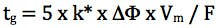
Where k* is the average gradient retention, ΔΦ is the change in %B (5% - 95% B = 0.9 for this equation), Vm is the column interstitial volume (π x radius2 x length x 0.6) and F is the flow rate (mL/min.).
So for a 50 x 2.1mm column at 0.2 mL/min and a gradient of 5 – 95% B, to obtain a k* value of 3 the gradient time would need to be;

One should note here that a value of 3 has been used for k* however the gradient slope (gradient time if we assume a fixed starting and ending composition) can be adjusted for values of k*
between 2 and 5. Some common column dimension / gradient slope combinations are shown in Table 4;
| Column Dimensions (mm) |
Flow Rate (mL/min.) |
Gradient Time (mins.) |
k*2 – k*5 (mins.) |
| 150 x 4.6 100 x 3.0 50 x 2.1 |
1.0 0.4 0.2 |
20 14 7 |
15.3 – 38.3 10.8 – 27.1 4.7 – 11.7 |
Table 4: Common conditions for HPLC screening with columns of various dimensions.
So, in practice we can now screen a range of stationary phase chemistries in columns with dimensions 50 x 2.1, 1.9mm (for example), using eluents with pH as close to 2, 4 and 6 as possible and the results of such an exercise are shown in Figure 2.

Figure 2: Stationary phase screen (C18 50 x 2.1 mm, 1.9 mm) of a test mix of 8 acidic, basic and neutral compounds using mobile phases of 0.1% v/v TFA (top), 10 mM ammonium formate (pH 4) and 10 mM ammonium acetate (pH 5.8). Gradient conditions 5 – 95% B Acetonitrile in 5 minutes.
Of course from Figure 2, one would go on to screen the same three pH values with Methanol as the organic modifier, making 6 experiments with each stationary phase. All 6 experiments would then be repeated using the various different stationary phases under investigation.
These chromatograms could then be assessed by eye, in combination with the efficiency, selectivity, peak shape and resolution values to assess which combination will be taken forward for optimisation, or if a different set of stationary phases or pH ranges may need to be employed.
If using computer optimisation software, the system will be able to predict, within limits, the optimum combination of variables and one will be able to assess if a usable set of conditions is obtainable with this set of stationary phases and pH range.
One final word on platform approaches of this type. It is easy to suffer poor efficiency due to poor peak shape of the analytes created by a mismatch between the sample diluent and the mobile phase under investigation. It is good practice to keep the eluotropic strength of the sample diluent as low as possible (low %B) and if possible (check the solubility of the analytes carefully), have 6 samples prepared in each of the 6 starting eluent compositions.
Related articles