02 Oct 2017
Calibration – done (badly?) every day
Many of our instrument techniques rely on a calibration in order to relate the detector response to the amount of analyte within our sample.
Where we have a wide expected analyte concentration range within our samples, it’s usual to achieve this using a range of standards of varying but known concentration to build a calibration curve of instrument response against known analyte amount. We then take the area count generated by the analyte from our sample (unknown) and interpolate the analyte amount or concentration using the calibration curve or, more precisely, using the regression equation which we derive from the calibration standard responses. Simple!
I’ve written about error estimation from the calibration curve and many others have written similar articles, however I continue to see mistakes being made in some of the crucial decisions associated with calibration curves, in particular with the treatment of the origin, weighting of the regression line, rejection of outliers and estimation of the ‘goodness of fit’ where we typically and often incorrectly rely upon the coefficient of determination (R2) to accept or reject the calibration function.
I’m not going to consider good practice for designing a calibration experiment such as the spacing of sample concentrations, the way in which the standards are prepared, the number of standards or the concentration range over which the calibrants are made. Further, I’m basing my treatment below on an experiments which uses absolute instrument response, rather than the response ratio obtained when using an internal standard to correct for variability in sample preparation or instrument response. There are excellent references which will guide you on these topics, including those in references X – Y below. [1-3]
For the first part of this discussion, I’m assuming that we are using a method that has already been validated and we are working on a multi-point calibration with a single replicate at each calibration level – which is typical of many validated methods in routine use where sample analyte concentration is expected to vary widely (in bioanalytical measurements, reaction monitoring or environmental analysis for example). I’ll show later that during validation, it’s essential to properly characterise the calibration function and test the validity of the regression model that we adopt. It is typical for analysts to construct a linear calibration curve of the form;

Equation 1.
where y is the detector response (area count for example), m is the slope of the regression line, x is the concentration and b is the y-intercept of the regression line. Typically, one might construct the curve, examine the R2 (coefficient of determination of the regression model) for it’s closeness to 1 and then carry on with our daily business. I’m often asked ‘how meaningful is the R2 value and what value should be considered as a rejection threshold for R2’ i.e. when is R2 too low and indicates that the instrument response or preparation of the calibration standards is ‘non-linear’ and should therefore not be used for the interpolation of analyte amounts from samples.
Experiment 1
Experiment 2
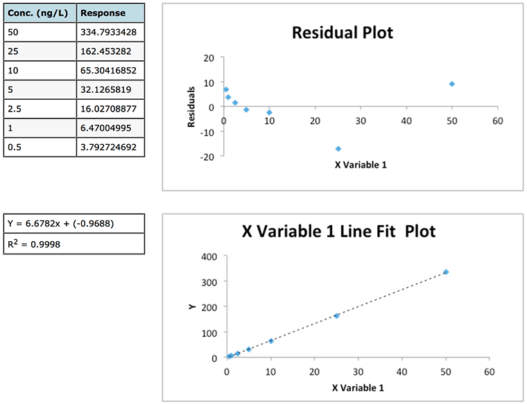
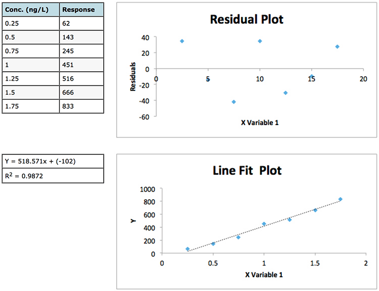
Figure 1: Data and residuals plots from two calibration experiments to illustrate the usefulness of residuals plots in determining the validity of linear regression model.
Whilst the regression data of experiment 1 looks a little ‘scruffy’ with low R2 value, large negative intercept (indicating bias or constant systematic error – of which more later) and large residuals, the residuals plot does show a good deal of random scatter – which is good. Whilst the regression data of experiment 2 looks much ‘better’ (high R2 value, small negative intercept and low absolute residuals), the residuals plot shows a somewhat typical ‘U’ shape that is common in analytical techniques where there is evidence of non-linear behaviour . One may predict that any data below 2.5 μg/mL will show a positive error (residual) and, arguably, that any data over around 40-50 μg/mL will also show a positive Y Residuals error. Similarly we could predict that sample concentrations between 10 and 40 μg/mL will show a negative residual. We are not supposed to be able to predict the errors when applying ordinary least squares (OSL) regression and as such we would need to question the data and goes some way to highlight that whilst data may show a high R2 value this does not necessarily mean a valid linear regression model is in play!
So we need to examine our data for heteroscedasticity (wow – scary statistical terms) and that may lead us to know something more about any statistical weighting that we may want to apply to the data. Which is another frequently asked question!
If weighting is to be applied, you probably want to have this justified using an F-test which examines the data for homo or heteroscedasticity – which is just a statistical term to describe if the data variances are equally random across the population (homo-) or show some bias to the higher or lower concentrations (hetero-).
This justification is often required, particularly when validating a method, by some regulatory authorities, such as the Food and Drug Administration (FDA) who state ‘Standard curve fitting is determined by applying the simplest model that adequately describes the concentration–response relationship using appropriate weighting and statistical tests for goodness of fit’. [5]
So fortunately, I had access to the gemfibrozil assay validation data and 6 replicate standard curves which were generated in order to assess various validation criteria and their back calculated values from the regression lines derived for each separate cure and these are shown in Table 1. We can use these data to get a better measure or picture of the homo- or heteroscedasticity of the data. Whilst I appreciate that one might not go these lengths when simply building a calibration curve using a previously validated assay – non-random residuals in a simple unweighted linear calibration do point towards a lack of attention to the proper calibration model during method development and validation.
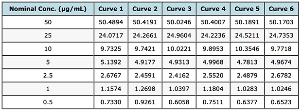
Table 1: Back calculated gemfibrozil concentrations for 6 separately prepared standard curves.
By combining all responses and concentrations into two contiguous columns with MS Excel and re-running the regression statistics described above we can get a fuller picture of the residuals spread for this particular analysis. The residuals plot shown in Figure 2 displays this data.
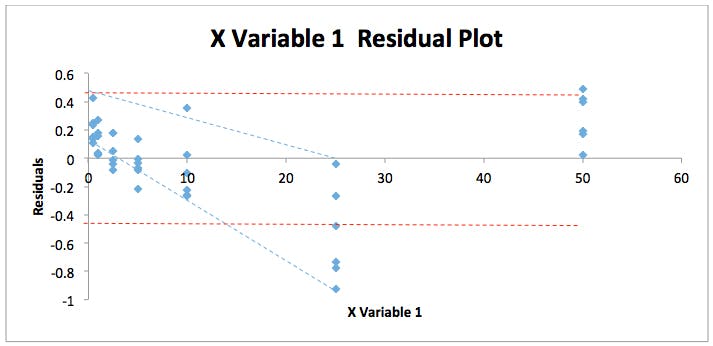
Figure 2: Residuals Plot for the back calculated gemfibrozil validation data in Table 1.
As can be seen the error in the data seems to form a ‘fan’ shape (blue dotted lines) which suggests that the variability in the data at low concentrations is lower than that at high concentrations rather than being equally and randomly distributed with equal variance – for instance between the two red dotted lines on the figure. However, it is difficult to be absolutely sure due to the distribution of the residuals – which we pointed out much earlier in the discussion, seems to take a U-shape. To test for heteroscedasticity and we can employ an F-test to test if this assumption is correct.
The null hypothesis (again just a statistical term to mean the assumption that we are testing) for this F- test is that the variance of the data at the low end of the curve and the high end of the curve are equal. This needs to be the case for unweighted linear regression to be the most appropriate model for our calibration.
An F-test can be easily carried out in MS Excel (F-Test Two-Sample for Variances) and works on the basis that if the F statistic value in the output is greater than the One-tail Critical F factor (take from tables or from the Excel output) then we need to reject the null hypothesis and state that the variances at the high and low end of the curve are unequal and that some form of weighting will produce more valid answers. The results of this test, performed on the instrument response rather than the interpolated values, are shown in Figure 3. As the F-test compares the variances of two samples (or populations if one has large amounts of data), it is typical to compare the data from the highest and lowest concentrations on the calibration curve. One needs at least two determinations at each concentration, although to increase the validity of the test – one should aim to have at least six replicates.
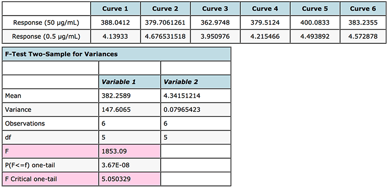
Figure 3: F test to investigate heteroscedasticity in calibration curve response data and justify the use of regression line weighting.
One very important point to note is that the data should be arranged such that the variance of variable 1 is larger than the variance of variable 2. If this is not the case, simply switch you data in their rows or columns prior to re-performing the F-test.
As F > F Critical one-tail (1853.09 > 5.050329), we reject the null hypothesis (original assumption that the variance of the data at the highest and lowest concentrations is equal) and conclude that the variances are unequal and therefore weighting of the calibration line may be appropriate.
This leads us nicely to the next frequently asked question of ‘what weighting do I apply to my calibration curve’.
We now start to need help from more advanced statistical techniques although an MS Excel spreadsheet with some simple embedded functions (caculations) will do the job very nicely. One very nice version that I regularly use can be found here
Download MS Excel spreadsheet of simple embedded functions here »
Whilst the effects of regression weighting are a little beyond the standard Excel Data Analysis toolpack, you will see that this modified sheet is very easy to use.
In the spreadsheet, enter your data (nominal concentration and average instrument response from Table 1) into the concentration and readings columns (B&C) and copy the relevant weighting from columns Z, AA into column A – these represent the weighting factors based your data for 1/x, 1/x2. Enter a value of 1 into column A for each concentration to the get the unweighted line (1/x0). Copy the same average instrument response data as you placed in column C into column J and column K will give you the interpolated (back calculated) value for the sample concentration. Then simply calculate the % recovery (Interpolated Conc. / Nominal Conc.) x 100 and for each value calculate the relative error (i.e. the difference between the calculated recovery and 100%).
I’ve shown these results in Table 2 for a calibration function based on the mean values of instrument response for the data in Table 1.
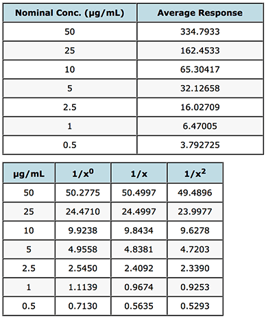
Interpolated Results from a single Calibration Curve
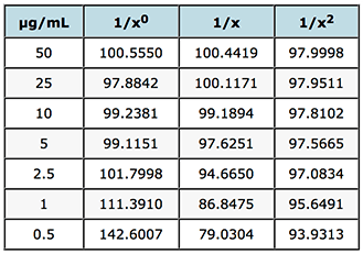
% recovery
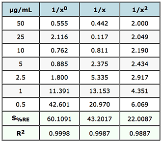
% Relative Error and Sum of % Relative Errors
Table 2: Evaluation of weighting factors on the quality of interpolated and back calculated data for an LCMS assay of gemfibrozil in human plasma.
The value of S%RE is the sum of the relative errors and gives a good indication of the most appropriate weighting to use on the data. In this case of weighting of 1/x2 will result in the smallest errors in the interpolated values of unknowns across the whole calibration range. If we refer back to the FDA guidelines mentioned above – it calls for the ‘simplest model’ to be used (1/x0 in preference to 1/x and then 1/x2 etc.) to ensure the data meets criteria on maximum allowable error – and of course we should examine the data carefully to see which of the weightings would fall into this category by referring to the allowable error in the particular guidelines chosen.
On visual inspection of the residuals data in Figure 2, it would appear that dropping the data associated with the 25ug/mL calibrant, may lead to a better overall result?
So the next frequently asked question is – ‘can I drop outliers from my data in order to improve the coefficient of determination and obtain more accurate results’.
I have to say this question is much more contentious and should only be considered after a thorough visual analysis of the calibration line and residuals. Where one point which lies way off the regression line and is causing ‘leverage’ or a skew of the data which obviously affects the slope of the calibration line (and often the accuracy of the interpolated data at the lowest concentrations) – then this process may be considered, but for no more than one point on the calibration line.
Grubb’s test can be used to determine whether or not a single outlying value within a set of measurements varies sufficiently from the mean value that it can be statistically classified as not belonging to the same population, and can therefore be omitted from subsequent calculations. As such, it is applied to either the highest or lowest residual value in the set; only one value may be omitted from the set on the basis of Grubb’s test.
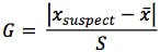
Where Xsuspect is the value with the largest or smallest ranked residual, x is the mean and S is the standard deviation of the residuals.
In practice, first obtain a regression of the calibration line, then rank the residuals for each calibration level (concentration) from highest to lowest prior to calculating the Grubb Factor for each. Again for this exercise I’ve used the mean response data which gave rise to the interpolated values in Table 1.
I’ve shown the data and results in Figure 4.
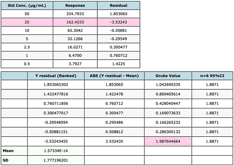
Figure 4: Grubs test for outliers on a gemfibrozil in human plasma.
Note that the Grubbs critical value is the two sided statistic at the 95% level of confidence.
In this case we note that because the Grubbs Factor value for the standard with residual -3.5324 (25 μg/mL point) is greater than the critical factor (1.887) then this point may be rejected from the calibration line and the quality of the interpolated data re-evaluated using the new regression equation.
Note again that this approach can only ever be applied to one point within the calibration curve and is used to prevent one outlier point from skewing the interpolated data. It goes without saying the underlying cause of the outlying point should be investigated in terms of integration of the chromatogram, instrument response, partial injection, sample preparation etc. in order that the causal issue can be avoided in future.
Now for our final frequently asked question – ‘do I include the origin in the calibration line?’
This is also a fairly controversial topic – however hopefully it’s one which is relatively easy to resolve.
Figure 5 shows a portion of the Regression Analysis carried out on the gemfibrozil analysis – the data is also shown in the Figure.
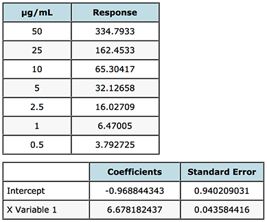
Figure 5: Assessment of the Standard Error of the Intercept, used to inform the decision on how the origin should be treated when generating the calibration model.
From Figure 5, the Intercept coefficient is the value of the intercept to be used in the regression equation and the Standard Error (SE) is the uncertainty associated with this value. If the magnitude (either positive or negative) of the intercept is greater than the standard error, this indicates that there is a bias in the data which cannot be explained by the regression model and the origin should not be included in the regression (i.e. the origin should not be forced).
In our case above the magnitude of the intercept and Standard Error are very close - -0.9688 and 0.9402 which gives us a dilemma, fortunately in the majority of cases the decision to include the origin or not is much less ambiguous. Our rule tells us that the intercept should not be forced on this occasion, however let’s just take a look at some data which quantifies the errors in the interpolation of data from regression lines created when ignoring, forcing or including the origin.
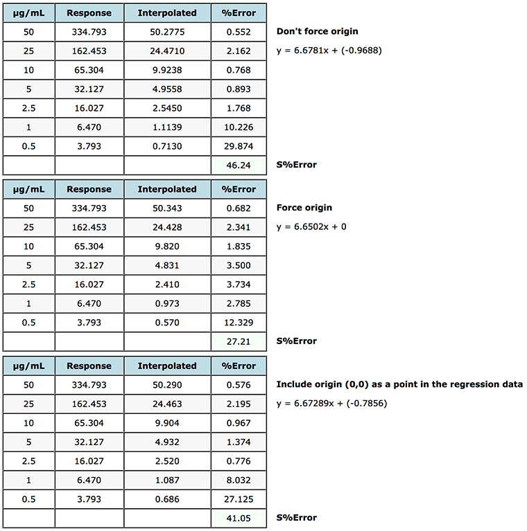
Figure 6: Assessment of various origin treatments on the % error of interpolated data when using simple linear regression.
As you can see from Figure 6, in this case forcing the origin (non-weighted linear regression was used) gives rise to increased error for lower concentrations but a lower error for the higher concentration standards, so one would need to take a view on the validity of the approach, as overall error (S%Error) the interpolated data across the whole range would be more accurate (S%error of 27.21 vs 46.24). Some software systems allow the origin to be ‘included’ as a point in the calibration table and will therefore use (0,0) as a datum when calculating the regression coefficients. As can be seen this makes only a very marginal difference in this case but should be considered when designing the calibration model. This should go alongside the injection of a ‘blank’ solution containing no analyte but which can be used to assess the contribution of co-eluting species or system noise on the calibration.
One may want to consider using a combination of 1/x2 weighting with forcing the origin to assess the impact on the quality of the interpolated data.
In conclusion to this very long entry – I have to state that I’m not a statistician, but that all of the information and data above uses approaches that I have ‘collected’ over the course of many years in analytical science and some very simple spreadsheet work – no professional statistics packages need to be used.
As usual, when I publish this sort of material, there will be sharp eyed chromatographers or statisticians who spot errors in the approaches or data. I welcome your feedback in this case and will follow up and cite all information that is received so that hopefully we can all do a little bit better with our calibration!
Related articles