13 Nov 2019
Measurements, Uncertainty, and Significant Figures

A calibrated piece of string. National Physical Laboratory, Teddington.
Errors
As separation scientists, an important part of our job is to make measurements. This is a simple enough statement. However, we should always bear in mind that every single measurement we make has some degree of ambiguity. Whether it’s because of instrument drift or poor calibration, because of the presence of interferences and artifacts, or because it is sometimes difficult to define exactly what we need to measure, we can never be sure that the value we obtain is the “true” value.
We are therefore forced to accept the existence of error. This error does not mean the measurement is wrong, it just means it has some degree of uncertainty, and it is also a very important part of our job to quantify and report this uncertainty. This article will try to give you some simple guidelines as to how to do this.
Reducing Uncertainty
Whilst acknowledging and reporting uncertainty is important, it is always desirable to reduce measurement error as much as possible within our equipment, time, and budgetary constraints. Well established good practices can help reduce uncertainty:
- Choose the best measuring instrument for the job
- Calibrate instruments and apply the corrections reported in the calibration certificate
- Use uncertainty budgets
- Compensate for any known errors
- Make calibrations traceable to national standards
- Be aware of error propagation in chain calibrations, serial dilutions, etc.
- Check calculations and manual data transfers
- Make repeat measurements
Accuracy (Inaccuracy) and Precision (Imprecision)

Figure 1: Accuracy versus precision.
Accuracy and precision are terms commonly used to describe measurement errors. Accuracy is defined by the International Organisation for Standardisation (ISO) as “the closeness of agreement between a test result and the accepted reference value”. This “reference” value, often represented by the Greek letter μ (mu), is akin to the “true” value. Given a series of replicate measurements, the average or arithmetic mean is calculated as:
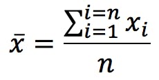
Imagine a hypothetical situation where we were able to measure something an infinite number of times. Taking an infinite number of replicate measurements would remove all possible uncertainty, and we could be completely confident of knowing the true value of whatever we were measuring. Statisticians call this infinite number of measurement replicates the Population and the mean of the population is, by definition, the true value . In the real world, however, my manager is unlikely to let me take an infinite number of measurements. Instead, I must content myself with a small number of replicates, a limited “subset” of the whole population.
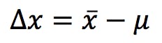
Statisticians call this a Sample and the limited size of this sample is, alas, the source of all my worries, errors and uncertainties. My measurement would be perfectly accurate if the mean (![]() ) and the reference (μ) were exactly the same value; but since the sample is only a subset of the population, the probability of this is vanishingly low. Inaccuracy, or lack of accuracy, is the difference between the two:
) and the reference (μ) were exactly the same value; but since the sample is only a subset of the population, the probability of this is vanishingly low. Inaccuracy, or lack of accuracy, is the difference between the two:
If only we could measure everything an infinite number of times! All our methods would be perfectly accurate, and we wouldn’t need to bother with validation and complicated statistics. We would also secure a job for life and solve unemployment!
Precision, the other big measure of uncertainty, indicates the agreement between repeat measurements. It is often reported as the standard deviation of the replicates:
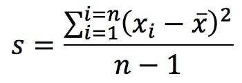
Spreadsheets and calculators have two alternative functions for standard deviation, and it is important to know which one to use. You get the calculation above when you press the following key in your calculator:

This formula gives the estimated standard deviation of the population based on the empirical measurements that make up our sample. The alternative calculation which is commonly found is:
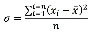
Note the different symbol (the Greek letter sigma) and that the denominator is n instead of n-1. This is the calculation you get when you press this key:

This second formula calculates the standard deviation of the sample itself; it does not attempt to estimate the standard deviation of the population. Since our objective is in general to characterise the population based on the knowledge gained from the sample, we must in most cases use the “σn-1” function. The “σn” function should be limited to those cases where the sample is the whole of the population (i.e. when there is nothing else for us to measure and there’s no need to make estimates), or when we have such a very large number of replicate measurements that both calculations converge.
Calculators, Spreadsheets, and Manual Calculations
Calculators and spreadsheets can produce results with a large number of significant figures, but all those decimal places do not always make sense. Below are some recommended practices for deciding how many significant figures we should carry, and for rounding up (or down) our results:
- The number of significant figures in any measurement is the number of digits which are known exactly, plus the digit whose value is uncertain.
- The result of a calculation cannot have more significant figures than the least certain measurement involved in the calculation.
Example: if the uncertainty in a measurement is in the second decimal place, it does not make sense to report the result with three or more decimal places, because we cannot be certain these additional figures are correct. - For additions and subtractions, the result is rounded to the last significant decimal place:

- For multiplications and divisions, the result is rounded to the lowest number of significant figures:
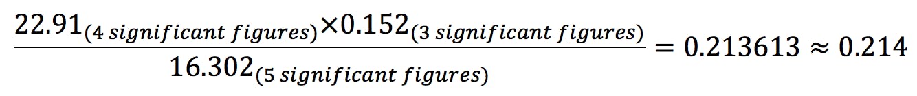
- It is good practice to carry all the decimal numbers allowed by the calculator or spreadsheet, and only round the final answer to the correct number of significant figures.
- If you must round intermediate results (for example, doing manual calculations) carry at least one more significant figure than required for the final result.
- Results are rounded up or down, depending on the nearest significant figure (see next section for the rules). Uncertainties, however, are always rounded up to the next figure, never down.
Rounding
Round the final answer to the correct significant figures using the following rules:
- If the digit that follows the significant digit is less than 5, round down:
12.442 ≈ 12.4 - If the digit that follows the significant figure is higher than 5, round up:
12.476 ≈ 12.5 - If the digit that follows the significant figure is exactly 5, round to the nearest even digit:
12.450 ≈ 12.4
12.550 ≈ 12.6
Significant Figures

We have explained that significant figures are the number of digits known to be correct, plus the digit whose value we are uncertain about. The following are some simple rules to calculate the number of significant figures:
- Trailing zeros (i.e. zeros to the right of a measurement) and zeros in the middle of the measurement do contribute to significant figures.
- Leading zeros (zeros to the left of a measurement) do not contribute to significant figures: they simply indicate the position of the decimal point. Example: the measurement 0.0120 g appears to have 5 significant figures. The last zero is indeed significant, as it indicates the uncertain digit. The first two zeros, however, are not significant. Expressing the measurement in scientific notation leaves no doubt that the number of significant figures is 3, rather than 5:
0.0120 = 1.20x10⁻²g - Logarithmic measurements (pH, pI, pO2, etc.) are a special case: The digits to the left of the decimal point indicate the power of 10, that is, the order of magnitude of the measurement. Therefore, they are not considered significant figures. Only the digits to the right of the decimal point (including any zeros immediately after the point) are considered significant figures. Example: the number of significant figures of pH 2.04 is two, not three.
Conclusions
As empirical scientists, our business is to collect good quality data and use it to interpret the world around us. We need to be mindful, however, of the limitations imposed on us by a range of external factors, such as the equipment we use, the protocols we follow, the nature of the systems we attempt to measure and, ultimately, the laws of probability (and managers, budgets, deadlines…)
The compounded effect of these factors is the introduction of errors in our measurements and uncertainty in the interpretation we make of them. We have tried to explore in simple terms why measurement uncertainty arises, and a few simple rules and best practices to try to mitigate or, at least, manage its effects.
There is ample literature on measurement error, uncertainty, and statistical analysis; and the subjects themselves are constantly evolving. We recommend some references for further reading:
- BIPM, IEC, IFCC, ILAC, ISO, IUPAC, IUPAP, OIML. International Vocabulary of Metrology – Basic and General Concepts and Associated Terms (VIM) Third Edition 2012.
- International Standard ISO/IEC 17025:2017 General Requirements for the competence of testing and calibration laboratories, Third Edition 2017, International Organization for Standardization, Geneva.
- Barwick, V., Ellison, S., Protocol for Uncertainty Evaluation from Validation Data, Version 5.1, January 2000, Valid Analytical Measurement (VAM) Project 3.2.1
- EURACHEM/CITAC Guide: Quantifying Uncertainty in Analytical Measurement, Third Edition 2012.
Related articles