Essential Detective Skills: Critical Evaluation of Chromatography Methods Part 2: GC

As with any profession, there really is no substitute for a lifetime of experience and the ‘school of hard knocks’ is a successful school indeed. However, the intention with this series is to condense some of these invaluable lessons into bitesize articles, which will help you to quickly gain the ability to critically evaluate your methods and link practical issues with methodological ‘quirks’.

This time we turn our attention to the gas chromatography (GC) method which I recently came across which was producing less than ideal results. I asked not to know anything of the problems, rather I was given the method to study in the hope that I could predict some of the issues and hopefully guide the analyst to a better performing method.

The method, outlined below, is for the analysis of a suite of barbiturate compounds in an extract from physiological matrices. Whilst there were several issues with the extraction method, consider only the chromatographic aspects here, leaving the evaluation of extraction methods for a future issue.

The Method

Column:           5% Phenyl Polydimethylsiloxane, 30 m x 0.25 mm, 0.25 µm

Carrier:             Hydrogen at 60 cm/s, measured at 60 °C

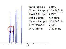
Oven:                60 °C, 60-150 °C at 25 °C/min, 170-300 °C at 10 °C/min

Injection:          Splitless, 250 °C, 1 min. purge time

Sample:            2µL of extract (isopropyl alcohol)

Detector*:        MS, 250 °C transfer line full scan at m/z 40-270

                           FID, 300 °C, Air 450 mL/min., Hydrogen 30 mL/min. Helium Makeup 50 mL/min.

*Capillary flow splitter with makeup to balance retention times between both detectors

So, where to start with the critical evaluation of a GC method such as this?

I always like to know the chemistry of the analytes. Figure 1 shows analyte structures for some of the target analytes in this method.

Figure 1: Selected barbiturate analytes from the analytical method under consideration

The barbiturate structures with their multiple aldehyde and amine groups would indicate that these relatively small analyte molecules would be reasonably polar in nature. The LogD value of Barbital, for example, is 0.6 at pH 7, falling to 0.1 at pH 8. The GC column stationary phase choice of 5% phenyl polydimethylsiloxane, however, if separation problems occur a more polar phase such as the 35% phenyl polydimethylsiloxane could be considered.

The analysis of structurally related target compounds often requires the use of longer and narrower bore GC columns, especially when using apolar phases, which tend to separate on analyte volatility. Where boiling points do not differ greatly, a stationary phase that can chemically discriminate between analytes should be considered, which seems to be the case for our analytes above. Once in the laboratory, if we discover that there is a poor resolution between analytes, apart from selecting a more highly polar stationary phase as discussed above, we may need to move to a longer (60m) column or reduce the column internal diameter, to drive the separation through improved efficiency rather than chemical means. A longer column will extend the analysis time and the use of 0.18mm internal diameter columns requires careful planning and reduced extra column volumes within the GC system. As the barbiturate analytes are not highly volatile, the relatively thin stationary phase film should be satisfactory.

For more information on GC column phase selection, go here.

Using hydrogen carrier gas with MS detection should always be considered as a potential issue, due to the vacuum at the outlet of the GC column leading to very low injector head pressure requirements. Consider the gas chromatograph head pressure requirements as very low values may lead to irreproducible retention times, separation variability, or even an inability for the instrument to attain or maintain a pressure setpoint. Whilst 60cm/sec is a reasonable linear velocity for hydrogen as a carrier gas with the column dimensions used in the method, due to the fact that we have a vacuum at the column outlet (i.e. the MS detector), the head pressure associated with this linear velocity under the method conditions is only around 2 psi. This may be difficult for the instrument gas pressure control systems to deliver in a reliable fashion, even though the quality and reliability of gas pressure/flow control units are very high in modern instruments.

Figure 2: Pressure and Flow Calculator used to assess the GC method under consideration [taken from Agilent website]

I used a manufacturer’s pressure/flow calculator to calculate the pressure required to achieve the desired linear velocity of the carrier gas under the method conditions ahead of even venturing into the laboratory. These tools are excellent for our critical evaluation toolkit, to evaluate and anticipate problems such as those described above. The use of wider bore capillary columns with low linear velocities, the use of hydrogen as a carrier gas, and the fact that MS detectors present us with a vacuum at the column outlet can all give rise to potential problems with low carrier gas outlet pressures. All these considerations can be investigated ahead of any practical work, using the type or pressure/flow calculator shown in Figure 2.

One further parameter, worthy of note, is the outlet flow which is shown in Figure 2. In this case, the flow is split between the mass spectrometer and an FID detector using a capillary flow splitting device, so we cannot assume that the full 1.1mL/min. of carrier gas reaches the spectrometer. However, this is not always the case, and it is worthwhile to ‘predict’ the outlet flow coming from the analytical column to ensure that it does not exceed the maximum for the spectrometer to be used. Even though modern vacuum pumps can withstand gas flows of 2 or even 4mL/min. of carrier gas flow (check the manufacturer’s flow or pressure limits for your instrument), it is always good practice to check the column outlet flow rate under your experimental combination of carrier gas type, pressure, and column dimensions. Exceeding the carrier gas flow limits will cause a noticeable reduction in the performance of the detector, especially in terms of the analyte ionisation characteristics (spectral appearance and/or analytical sensitivity) and may even cause the instrument to shut down. Also bear in mind that the use of hydrogen carrier may require adjustments to the MS instrument hardware and may result in changes to the spectra of certain analyte types. For further information on the use of hydrogen with MS detectors, go here.

When using splitless injection, it is typical to start the oven temperature program at around 20oC below the boiling point of the sample solvent, to ensure good thermal focusing of the analyte at the head of the analytical column and therefore sharp rather than broad or split peaks. In this case, the solvent is isopropyl alcohol with a boiling point of around 82oC and an oven starting temperature of 60oC seems appropriate in this case and we would assume that certainly, the earlier eluting peaks within the chromatogram should be ‘sharp’ from a chromatographic perspective. This so-called ‘solvent focussing’ phenomenon applies mainly to earlier eluting species as it is assumed that the more volatile analytes will remain associated with the injection solvent vapour when transitioning from the inlet into the analytical column. If the starting oven temperature were any higher, the solvent containing the analyte molecules would be unable to condense onto the inner walls of the capillary column which is the basis of the solvent focusing effect, and peak shape broadening, or deformation could occur. It should also be noted that it is usual practice to hold the initial oven temperature to allow optimum peak focussing through both thermal and solvent effects. In this method, there is no initial hold time, and this can potentially lead to peak shape deformation (typically peak splitting/tailing) and issues with peak area reproducibility. Consider the introduction of an isothermal period that initially matches the purge time (see below) and which can be empirically optimised by extending or shortening the hold time, to overcome any peak shape issues.

There are two further important considerations when investigating potential issues with a new method that uses splitless injection; the injection volume as well as the splitless or purge time associated with the injection phase. Splitless injection, as you may be aware, is used when we need to introduce all, or the vast majority, of our sample into the GC column to obtain the required sensitivity when analytes are present at very low concentrations. To achieve this, during the first part of the injection phase, the split valve is closed, and all of the sample vapour produced in the inlet are passed to the column. After a pre-defined time, the split valve is opened, and any residual solvent/sample vapours are vented from the inlet to avoid large/tailing solvent peaks and rising baselines as well as to protect the inlet from contamination. It is important that during the splitless phase of the analysis, the volume of sample vapours generated does not exceed the available volume within the inlet (predominantly defined by the internal volume of the inlet liner). If the inlet volume is exceeded, a process colloquially known as backflash can occur, which may lead to deposition of analyte within the gas supply and outlet lines leading into and out of the inlet, which ultimately risks carryover and problems with quantitative reproducibility.

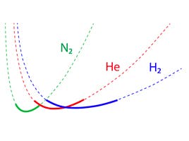
Figure 3: Vapour volume calculator used to assess the possibility of backflash during injection [taken from Agilent website]

Access our Vapour Volume Calculator on CHROMacademy.

Find it amongst other interactive GC tools. 

Again, I have used a helpful tool to predict the vapour volume created under the conditions used in our method. Figure 3 shows that the 2µL injection under the inlet conditions selected is dangerously close to the total volume of the liner chosen. If issues with carry-over are encountered when implementing the method, consider reducing the injected volume if sensitivity requirements can still be met. Alternatively, consider a pressure pulsed injection, where the inlet pressure is raised during the injection to constrict the expansion of the sample vapour. This will avoid backflashing the solvent vapour, whilst retaining the 2µL sample injection size.

For a more comprehensive treatment of optimising splitless injection conditions with pressure pulsed injection, see this link.

The purge, or splitless, time corresponds to the time at which the split vent is opened to release any lingering vapours and needs to be optimised empirically. Typically, one would begin with a shorter purge time (30 secs. would be typical) and the purge time lengthened until the peak area of analytes stabilises. Too short a purge time leads to analytes, which have not passed into the column, being lost from the split line. Typically, the analyte peak area will stabilise and remain constant, and the purge time should be increased in 10 – 15 second increments until the peak area stabilises and the purge time set to the value which corresponds to the second time increment where peak area remains stable. The 1-minute purge time within the method seems reasonable. However, if the solvent peak tails or the baseline is noisy and rises dramatically throughout the analysis, one may consider reducing the purge time.

Without seeing a chromatogram, it is very difficult to predict the suitability of the temperature program gradient. However, when analytes are very similar in chemistry (homologs etc.), the rule of thumb is that lower ramp rates tend to work better. The 25oC ramp rate at the start of the analysis should be carefully considered if problems with selectivity/resolution are encountered. However, as the gradient program in our method slows to 10oC per minute from 170oC, then I suspect that any problematic analyte peak pairs occur from 4 minutes onwards within the chromatogram and the rapid initial program is merely used to reduce overall analysis time. If there’s a need to further optimise the oven temperature gradient, then many good tips can be found at this link.

In terms of the Flame Ionisation Detector (FID) parameters, the absolute values for temperature and gas flow rates will vary by manufacturer, again though, we can highlight some general principles. It is usual to keep the detector temperature elevated above the final oven temperature, to prevent condensation effects. One should consider raising the detector temperature from 300oC to 325 or 350oC to prevent water condensation in the detector which reduces sensitivity and reduces the risk of analyte deposition within the detector body. The gas flow settings within the method seem reasonable, although most methods tend to have similar gas flow for the fuel (hydrogen) and make-up (helium) gas flows, typically because they have not been optimised to obtain the best sensitivity. In our example, the make-up flow is higher than the fuel gas flow, but this may well be because the method has been optimised. If not, we should consider reducing the make-up gas flow. Typically, the air to fuel gas ratio would be around 10:1 and in the method cited the ratio is a little higher. Again, if sensitivity needs to be improved, consider lowering the airflow rate or slightly increasing the fuel gas flow. However, these recommended settings are somewhat manufacturer dependant.

The MSD transfer line is a heated line that carries the column effluent from the oven to the ion source within the detector. The temperature of the transfer line should be set to avoid condensation of analytes within the heated region, which may result in reduced method sensitivity and carry-over. It is recommended that the transfer line temperature should not be more than 20oC below the oven temperature and therefore, in our method, we should consider raising the transfer line temperature to at least 280oC. No further details are given regarding the other MS parameter settings, which is an omission in the method specification. For brevity, we will consider a critical evaluation of MS detector settings in a future blog entry.

Who would have thought that there was so much to discuss from a few simple Gas Chromatography method settings!? The skill in critical evaluation of methods is to be prepared, almost to predict issues before they occur. This method may work perfectly well in practice; however, undertaking this short evaluation exercise will allow us to prepare for any problems, and to prioritise the adjustments we might make if specific issues arise.